2. One-way ANOVA in a RCBD

To install and load all the packages used in this chapter, run the following code:

for (pkg in c("desplot", "emmeans", "ggtext", "here", "multcomp", "multcompView", "tidyverse")) {
  if (!require(pkg, character.only = TRUE)) install.packages(pkg)
}

library(desplot)
library(emmeans)
library(ggtext)
library(here)
library(multcomp)
library(multcompView)
library(tidyverse)

From CRD to RCBD

In the previous chapter, we analyzed data from a melon variety trial using a completely randomized design (CRD). In a CRD, treatments are randomly assigned to experimental units (plots) without any restrictions. While this is the simplest design, it assumes that all experimental units are equally variable.

However, in agricultural experiments, we often face situations where our experimental units are not homogeneous:

• Fields may have gradients in soil fertility
• Greenhouse benches may differ in light or temperature exposure
• Laboratory work may span multiple days with different conditions

Why Use Blocking?

A Randomized Complete Block Design (RCBD) addresses this by grouping experimental units into “blocks” where units within each block are more similar to each other than to units in other blocks. Then, each treatment appears exactly once in each block (hence “complete” block design).

The advantages of blocking include:

1. Increased precision: By accounting for known sources of variation via the blocks, we reduce unexplained variation (noise/error)
2. Better estimates: As a result, treatment effects are estimated more precisely
3. Valid comparisons: Each treatment faces the same set of conditions across blocks

Think of it this way: In a CRD, all variation is either explained by treatments or considered random error. In an RCBD, all variation is either explained by treatments or by blocks, leaving less unexplained variation.

Data

For this example, we’ll use data from a cultivar trial reported by Clewer & Scarisbrick (2001). The experiment tested four cultivars in three blocks. The response variable is yield (t/ha).

dat <- read_csv(here("data", "ClewerScarisbrick2001.csv"))
dat

Rows: 12 Columns: 5
── Column specification ────────────────────────────────────────────────────────
Delimiter: ","
chr (2): block, cultivar
dbl (3): yield, row, col

ℹ Use `spec()` to retrieve the full column specification for this data.
ℹ Specify the column types or set `show_col_types = FALSE` to quiet this message.

# A tibble: 12 × 5
   block cultivar yield   row   col
   <chr> <chr>    <dbl> <dbl> <dbl>
 1 B1    C1         7.4     2     1
 2 B1    C2         9.8     3     1
 3 B1    C3         7.3     1     1
 4 B1    C4         9.5     4     1
 5 B2    C1         6.5     1     2
 6 B2    C2         6.8     4     2
 7 B2    C3         6.1     3     2
 8 B2    C4         8       2     2
 9 B3    C1         5.6     2     3
10 B3    C2         6.2     1     3
11 B3    C3         6.4     3     3
12 B3    C4         7.4     4     3

The dataset contains:

• cultivar: Four cultivars labeled C1 through C4
• block: Three blocks labeled B1 through B3
• yield: Crop yield in tons per hectare
• row and col: Field plot coordinates for visualization via desplot

Format

As with the previous analysis, we need to ensure our categorical variables are properly formatted as factors. Here, this means formatting two variables: block and cultivar. Below are two different way to do this.

# Option 1: mutate(... , ...)
dat <- dat %>%
  mutate(
    block = as.factor(block),
    cultivar = as.factor(cultivar)
  )

# Option 2: mutate(across(...))
dat <- dat %>%
  mutate(across(c(block, cultivar), ~ as.factor(.x)))

dat

# A tibble: 12 × 5
   block cultivar yield   row   col
   <fct> <fct>    <dbl> <dbl> <dbl>
 1 B1    C1         7.4     2     1
 2 B1    C2         9.8     3     1
 3 B1    C3         7.3     1     1
 4 B1    C4         9.5     4     1
 5 B2    C1         6.5     1     2
 6 B2    C2         6.8     4     2
 7 B2    C3         6.1     3     2
 8 B2    C4         8       2     2
 9 B3    C1         5.6     2     3
10 B3    C2         6.2     1     3
11 B3    C3         6.4     3     3
12 B3    C4         7.4     4     3

Explore

Let’s first examine the summary statistics by both cultivar and block to understand the data structure:

# Summary by cultivar
dat %>%
  group_by(cultivar) %>%
  summarize(
    count = n(),
    mean_yield = mean(yield),
    sd_yield = sd(yield),
    min_yield = min(yield),
    max_yield = max(yield)
  ) %>%
  arrange(desc(mean_yield))

# A tibble: 4 × 6
  cultivar count mean_yield sd_yield min_yield max_yield
  <fct>    <int>      <dbl>    <dbl>     <dbl>     <dbl>
1 C4           3        8.3    1.08        7.4       9.5
2 C2           3        7.6    1.93        6.2       9.8
3 C3           3        6.6    0.624       6.1       7.3
4 C1           3        6.5    0.9         5.6       7.4

# Summary by block
dat %>%
  group_by(block) %>%
  summarize(
    count = n(),
    mean_yield = mean(yield),
    sd_yield = sd(yield),
    min_yield = min(yield),
    max_yield = max(yield)
  ) %>%
  arrange(desc(mean_yield))

# A tibble: 3 × 6
  block count mean_yield sd_yield min_yield max_yield
  <fct> <int>      <dbl>    <dbl>     <dbl>     <dbl>
1 B1        4       8.5     1.33        7.3       9.8
2 B2        4       6.85    0.819       6.1       8  
3 B3        4       6.4     0.748       5.6       7.4

We see that:

• Cultivar C4 has the highest mean yield
• Block B1 has notably higher yields than B2 and B3

Just to be clear: Everything seems to be growing better in block B1. This is not a cultivar effect - it’s a block effect. It cannot be because of a cultivar, because all cultivars are present in each block. This is exactly why we use blocking - there are systematic differences between blocks that we want to account for.

Let’s visualize the data to see the relationship between cultivars and blocks:

ggplot(data = dat) +
  aes(y = yield, x = cultivar, color = block) +
  geom_point() +
  scale_x_discrete(
    name = "Cultivar"
  ) +
  scale_y_continuous(
    name = "Yield",
    limits = c(0, NA),
    expand = expansion(mult = c(0, 0.1))
  ) +
  scale_color_discrete(
    name = "Block"
  ) +
  theme_classic()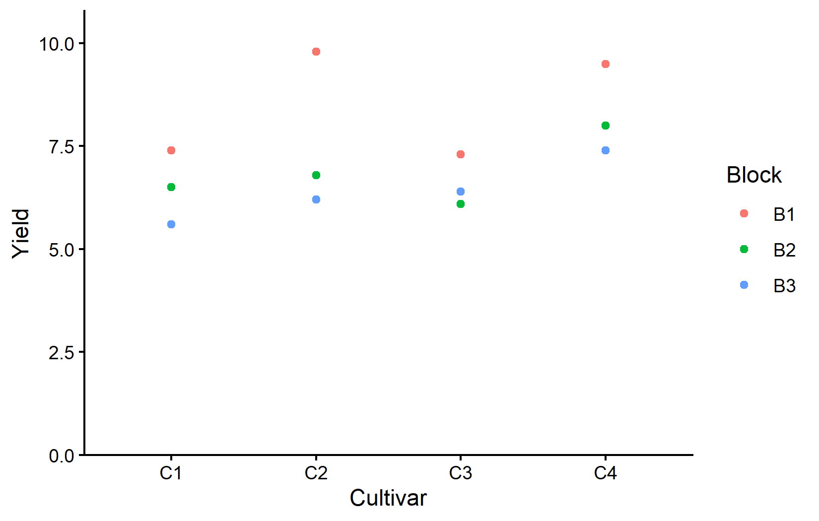

This plot shows how yields vary both by cultivar (x-axis) and block (color). Notice every cultivar had its highest yield in block B1. This is once again a clear indication of the block effect. Something about block B1 is making everything grow better.

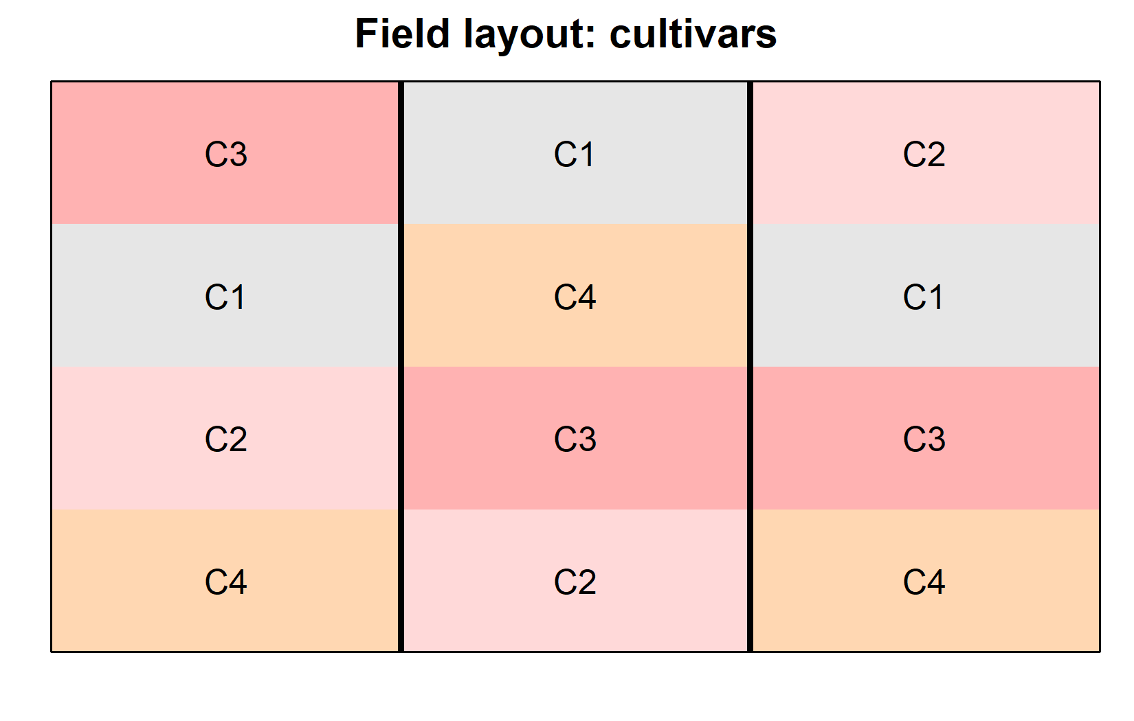
Now let’s visualize the experimental layout to understand the physical arrangement:

desplot(
  data = dat,
  flip = TRUE, # row 1 on top, not on bottom
  form = cultivar ~ col + row, # fill color per cultivar
  out1 = block, # line between blocks
  text = cultivar, # cultivar names per plot
  cex = 1, # cultivar names: font size
  shorten = FALSE, # cultivar names: don't abbreviate
  main = "Field layout: cultivars", # plot title
  show.key = FALSE # hide legend
)

desplot(
  data = dat,
  flip = TRUE, # row 1 on top, not on bottom
  form = yield ~ col + row, # fill color according to yield
  out1 = block, # line between blocks
  text = cultivar, # cultivar names per plot
  cex = 1, # cultivar names: font size
  shorten = FALSE, # cultivar names: don't abbreviate
  main = "Yield per plot", # plot title
  show.key = FALSE # hide legend
)

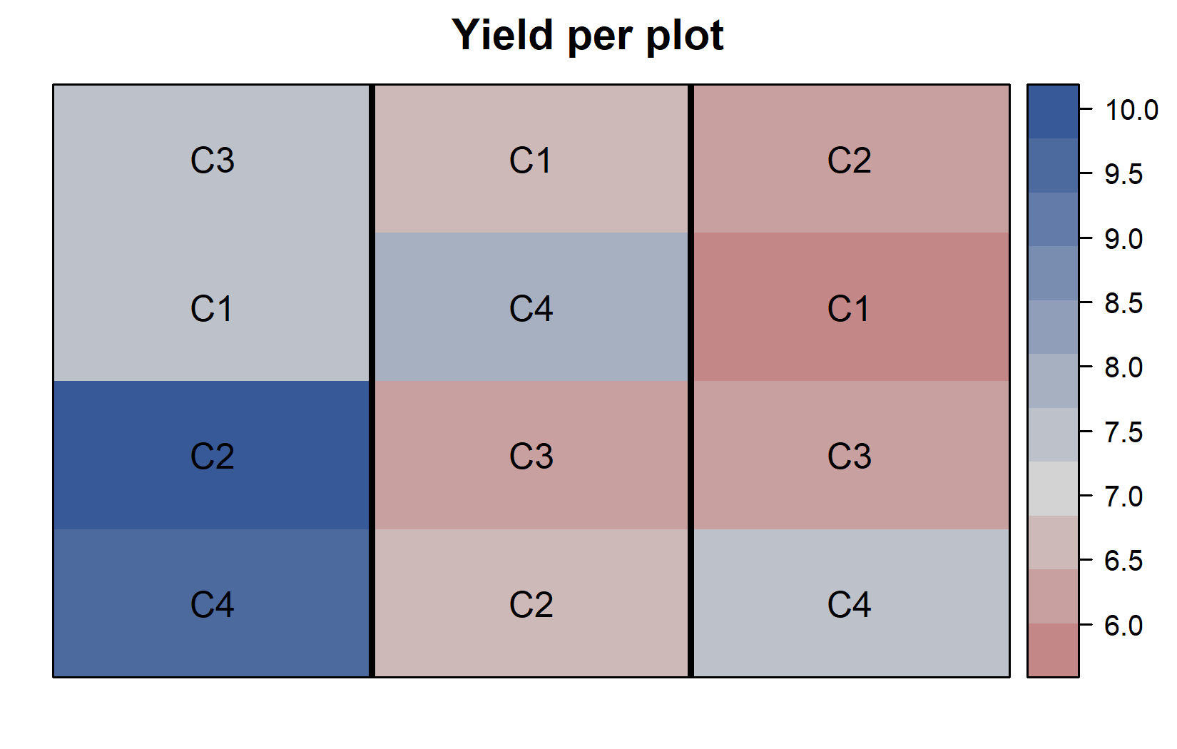
The field layouts confirm:

1. Each cultivar appears exactly once in each block (complete block design)
2. Block B1 (left) has generally higher yields than the other blocks
3. Within each block, cultivar C4 has either the highest or second highest yield compared to the other cultivars

Model and ANOVA

Understanding the RCBD Model

The key difference between CRD and RCBD in terms of model formulation is an additional effect for blocks. In a CRD, we only include the treatment effect:

yield ~ cultivar

In an RCBD, we add the block effect:

yield ~ cultivar + block

Let’s fit this model:

mod <- lm(yield ~ cultivar + block, data = dat)
mod

Call:
lm(formula = yield ~ cultivar + block, data = dat)

Coefficients:
(Intercept)   cultivarC2   cultivarC3   cultivarC4      blockB2      blockB3  
       7.75         1.10         0.10         1.80        -1.65        -2.10  

Notice that the coefficients now include both cultivar and block effects and both are once again “missing” their first level. The block effects (blockB2 and blockB3) are both negative, indicating lower yields in these blocks compared to block B1 (the reference level set to 0). The cultivar effects (cultivarC2, cultivarC3, and cultivarC4) are all positive, indicating higher yields compared to cultivar C1 (the reference level set to 0). This, however, is coincidence, as these levels are not sorted in any particular order and it is always the first level that is set to 0.

The good news is, that everything from here on is the same as in the CRD analysis. We can still use the anova() function to conduct an ANOVA on this model, and we can still use emmeans() to get estimated marginal means (adjusted means) for our cultivars. Besides our factor being called cultivar instead of variety, we do not even need to change the code from the previous chapter. The important change is that we now have included the block effect in our model. The ANOVA table will therefore also include the block effect. The adjusted means - or rather their standard errors - will also be adjusted for the block effect.

WarningModel assumptions met?

It is at this point (i.e. after fitting the model and before interpreting the ANOVA) that one should check whether the model assumptions are met. Find out more in Appendix A1: Model Diagnostics.

Conducting the ANOVA

ANOVA <- anova(mod)
ANOVA

Analysis of Variance Table

Response: yield
          Df Sum Sq Mean Sq F value   Pr(>F)   
cultivar   3   6.63    2.21   5.525 0.036730 * 
block      2   9.78    4.89  12.225 0.007651 **
Residuals  6   2.40    0.40                    
---
Signif. codes:  0 '***' 0.001 '**' 0.01 '*' 0.05 '.' 0.1 ' ' 1

In this ANOVA table:

1. Both effects appear in the table: cultivar and block
2. Both cultivar (p < 0.05) and block (p < 0.05) effects are statistically significant

The block effect being statistically significant confirms that blocking was beneficial - we reject the null hypothesis that there is no difference between blocks. Thus, by including the block effect in our model, we accounted for this variation, which would otherwise have been attributed to error/unexplained noise. Even though we’re primarily interested in cultivar effects, including the block effect improves our analysis.

The cultivar effect being statistically significant indicates that at least one cultivar is different from the others. This is of course our main interest. We can now proceed to post-hoc comparisons to identify which cultivars are significantly different from each other.

Mean Comparisons

As in the CRD analysis, we use estimated marginal means (emmeans) for post-hoc comparisons:

mean_comp <- mod %>%
  emmeans(specs = ~ cultivar) %>% # adj. mean per cultivar
  cld(adjust = "none", Letters = letters) # compact letter display (CLD)

mean_comp

 cultivar emmean    SE df lower.CL upper.CL .group
 C1          6.5 0.365  6     5.61     7.39  a    
 C3          6.6 0.365  6     5.71     7.49  a    
 C2          7.6 0.365  6     6.71     8.49  ab   
 C4          8.3 0.365  6     7.41     9.19   b   

Results are averaged over the levels of: block 
Confidence level used: 0.95 
significance level used: alpha = 0.05 
NOTE: If two or more means share the same grouping symbol,
      then we cannot show them to be different.
      But we also did not show them to be the same. 

Note that these means are adjusted for block effects. In a balanced design like this (each cultivar appears once in each block), the adjusted means are the cultivar averages across blocks. The emmeans approach accounts for the block structure when calculating standard errors.

Visualizing Results

As the final step in this material, let’s create a comprehensive plot that shows both the raw data and the statistical results. To understand each component of the plot, please have a look at this chapter’s video.

my_caption <- "Black dots represent raw data.
Red dots and error bars represent adjusted means with 95% confidence
limits per cultivar. Means followed by a common letter are not
significantly different according to Fisher's LSD test."

ggplot() +
  aes(x = cultivar) +
  # black dots representing the raw data
  geom_point(
    data = dat,
    aes(y = yield, shape = block)
  ) +
  # red dots representing the adjusted means
  geom_point(
    data = mean_comp,
    aes(y = emmean),
    color = "red",
    position = position_nudge(x = 0.1)
  ) +
  # red error bars representing the confidence limits of the adjusted means
  geom_errorbar(
    data = mean_comp,
    aes(ymin = lower.CL, ymax = upper.CL),
    color = "red",
    width = 0.1,
    position = position_nudge(x = 0.1)
  ) +
  # red letters
  geom_text(
    data = mean_comp,
    aes(y = emmean, label = str_trim(.group)),
    color = "red",
    position = position_nudge(x = 0.2),
    hjust = 0
  ) +
  scale_x_discrete(
    name = "Cultivar"
  ) +
  scale_y_continuous(
    name = "Yield",
    limits = c(0, NA),
    expand = expansion(mult = c(0, 0.1))
  ) +
  scale_shape_discrete(
    name = "Block"
  ) +
  theme_classic() +
  labs(caption = my_caption) +
  theme(plot.caption = element_textbox_simple(margin = margin(t = 5)),
        plot.caption.position = "plot")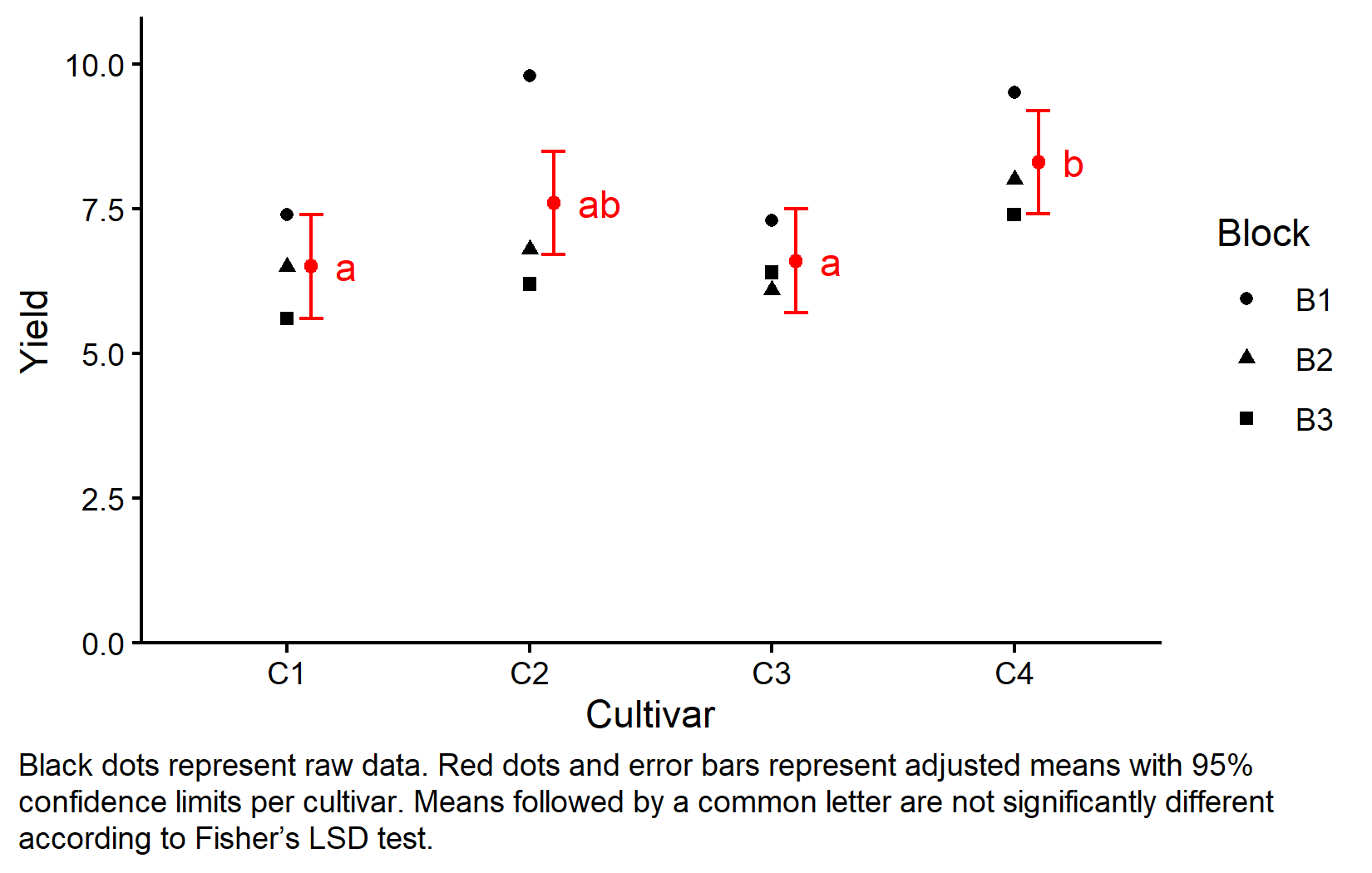

CRD vs RCBD Comparison

Let’s summarize the key differences between our CRD and RCBD analyses:

1. Model formula:
   • CRD: yield ~ cultivar
   • RCBD: yield ~ cultivar + block
2. Sources of variation:
   • CRD: Treatment and residual error
   • RCBD: Treatment, blocks, and residual error
3. Precision:
   • CRD: All unexplained variation goes to error
   • RCBD: Block variation is removed from error, increasing precision
4. When to use:
   • CRD: When experimental units are homogeneous
   • RCBD: When there are known sources of heterogeneity

Wrapping Up

You’ve now learned how to analyze data from a randomized complete block design, building upon the concepts from the completely randomized design. Blocking is a powerful tool that increases the precision of your experiments when dealing with heterogeneous experimental conditions.

NoteKey Takeaways

1. Randomized Complete Block Design (RCBD) groups similar experimental units into blocks, reducing unexplained variation.

2. Blocking improves precision by accounting for known sources of variation, making treatment comparisons more accurate.

3. The RCBD model includes both treatment and block effects: response ~ treatment + block.

4. ANOVA for RCBD tests both treatment and block effects, though we’re primarily interested in treatments.

5. Estimated marginal means in RCBD are adjusted for block effects, providing better treatment comparisons.

This concludes our introduction to analyzing experimental designs. You now have the tools to handle both simple (CRD) and more complex (RCBD) experimental layouts using ANOVA and mean comparison techniques in R.