6. One-way ANOVA in a Row-Column Design

To install and load all the packages used in this chapter, run the following code:

for (pkg in c("agridat", "desplot", "emmeans", "ggtext", "here", "lme4", 
              "lmerTest", "multcomp", "multcompView", "tidyverse")) {
  if (!require(pkg, character.only = TRUE)) install.packages(pkg)
}

library(agridat)
library(desplot)
library(emmeans)
library(ggtext)
library(here)
library(lme4)
library(lmerTest)
library(multcomp)
library(multcompView)
library(tidyverse)

Row-Column Designs

In Chapter 3, we encountered the Latin Square design, which controls for two sources of variation (rows and columns) simultaneously. However, the Latin Square has a major limitation: the number of treatments must equal the number of rows and columns. This makes it impractical for experiments with many treatments.

What is a Row-Column Design?

A resolvable row-column design extends the Latin Square concept to accommodate more treatments. Like an alpha design, it has complete replicates that are subdivided - but here each replicate is subdivided into both incomplete rows and incomplete columns. This provides double blocking within each replicate.

The key features are:

1. Two-dimensional blocking: Each replicate has both row and column structure
2. Incomplete blocks: Neither rows nor columns contain all treatments
3. Resolvability: Replicates are complete, containing each treatment exactly once
4. Flexibility: Can accommodate various numbers of treatments

The advantages include:

1. Control of two gradients: Accounts for spatial trends in two directions simultaneously
2. More treatments than Latin Square: Not limited to t×t arrangements
3. Increased precision: Double blocking can substantially reduce experimental error
4. Practical for field trials: Matches the rectangular layout of many field experiments

Data

This example considers data published in Kempton, Fox, and Cerezo (1997) from a yield trial laid out as a resolvable row-column design. The trial had 35 genotypes (gen), 2 complete replicates (rep) with 5 rows (row) and 7 columns (col) each. Thus, each replicate forms a 5×7 grid with incomplete rows and columns.

Import

The data is available as part of the {agridat} package:

dat <- as_tibble(agridat::kempton.rowcol)
dat

# A tibble: 68 × 5
   rep     row   col gen   yield
   <fct> <int> <int> <fct> <dbl>
 1 R1        1     1 G20    3.77
 2 R1        1     2 G04    3.21
 3 R1        1     3 G33    4.55
 4 R1        1     4 G28    4.09
 5 R1        1     5 G07    5.05
 6 R1        1     6 G12    4.19
 7 R1        1     7 G30    3.27
 8 R1        2     1 G10    3.44
 9 R1        2     2 G14    4.3 
10 R1        2     4 G21    3.86
# ℹ 58 more rows

The dataset contains:

• rep: Two complete replicates (R1, R2)
• row: Row position within replicate (1-5)
• col: Column position within replicate (1-7)
• gen: 35 genotypes
• yield: Crop yield

Note that there are missing values in this dataset - two plots have no yield recorded.

Format

For our analysis, gen should be encoded as a factor. We also create factor versions of row and col for the statistical model:

dat <- dat %>%
  mutate(
    gen = as.factor(gen),
    rowF = as.factor(row),
    colF = as.factor(col)
  )

dat

# A tibble: 68 × 7
   rep     row   col gen   yield rowF  colF 
   <fct> <int> <int> <fct> <dbl> <fct> <fct>
 1 R1        1     1 G20    3.77 1     1    
 2 R1        1     2 G04    3.21 1     2    
 3 R1        1     3 G33    4.55 1     3    
 4 R1        1     4 G28    4.09 1     4    
 5 R1        1     5 G07    5.05 1     5    
 6 R1        1     6 G12    4.19 1     6    
 7 R1        1     7 G30    3.27 1     7    
 8 R1        2     1 G10    3.44 2     1    
 9 R1        2     2 G14    4.3  2     2    
10 R1        2     4 G21    3.86 2     4    
# ℹ 58 more rows

Explore

Let’s examine the summary statistics by genotype:

dat %>% 
  group_by(gen) %>% 
  summarize(
    count = n(),
    mean_yield = mean(yield, na.rm = TRUE),
    sd_yield = sd(yield, na.rm = TRUE)
  ) %>%
  arrange(desc(mean_yield))

# A tibble: 35 × 4
   gen   count mean_yield sd_yield
   <fct> <int>      <dbl>    <dbl>
 1 G19       2       6.07   1.84  
 2 G07       2       5.74   0.976 
 3 G33       2       5.13   0.820 
 4 G06       2       4.96   0.940 
 5 G09       2       4.94   1.68  
 6 G11       2       4.93   1.03  
 7 G14       2       4.92   0.877 
 8 G27       2       4.89   1.80  
 9 G03       2       4.78   0.0424
10 G25       2       4.78   0.361 
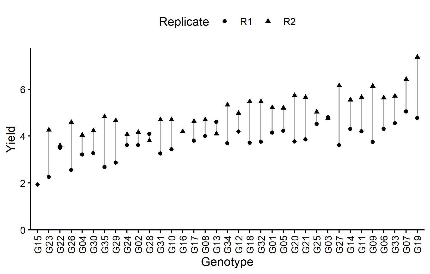
# ℹ 25 more rows

Most genotypes appear twice (once per replicate), but some have only one observation due to missing data. Let’s visualize the data:

# sort genotypes by mean yield
gen_order <- dat %>% 
  group_by(gen) %>% 
  summarise(mean = mean(yield, na.rm = TRUE)) %>% 
  arrange(mean) %>% 
  pull(gen) %>% 
  as.character()

ggplot(data = dat) +
  aes(
    y = yield,
    x = gen,
    shape = rep
  ) +
  geom_line(
    aes(group = gen),
    color = "darkgrey"
  ) +
  geom_point() +
  scale_x_discrete(
    name = "Genotype",
    limits = gen_order
  ) +
  scale_y_continuous(
    name = "Yield",
    limits = c(0, NA),
    expand = expansion(mult = c(0, 0.05))
  ) +
  scale_shape_discrete(
    name = "Replicate"
  ) +
  guides(shape = guide_legend(nrow = 1)) +
  theme_classic() +
  theme(
    legend.position = "top", 
    axis.text.x = element_text(angle = 90, vjust = 0.5)
  )

Now let’s look at the field layout. Note that the two missing plots will appear as white/empty:

desplot(
  data = dat,
  form = gen ~ col + row | rep, # fill color per genotype, panels per replicate
  text = gen, 
  cex = 0.7, 
  shorten = FALSE,
  out1 = row, out1.gpar = list(col = "black"), # lines between rows
  out2 = col, out2.gpar = list(col = "black"), # lines between columns
  main = "Field layout", 
  show.key = FALSE
)     

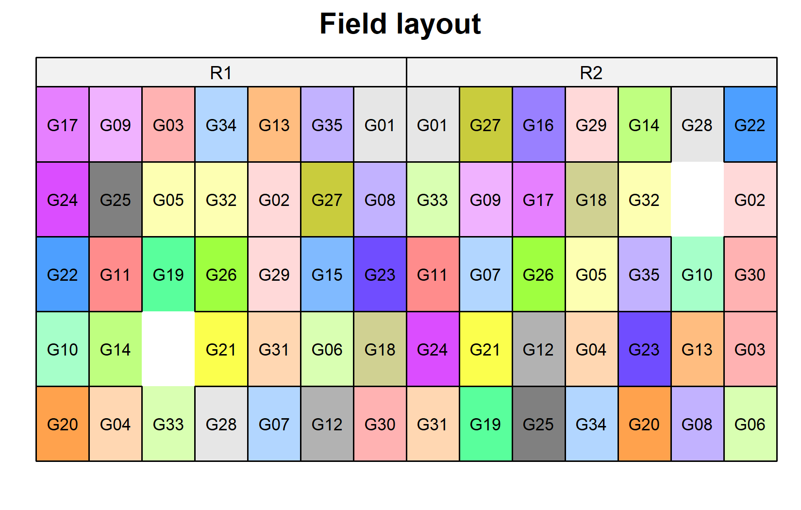
The black lines show the row and column structure within each replicate. Each genotype appears once per replicate, but in different row-column positions.

Model and ANOVA

Choosing Between Fixed and Random Effects

For a row-column design, the model needs to account for row and column effects within each replicate. We can treat these as either fixed or random effects. Let’s compare both approaches:

# Rows and columns as fixed effects
mod_fixed <- lm(yield ~ gen + rep + rep:rowF + rep:colF,
                data = dat)

# Rows and columns as random effects
mod_random <- lmer(yield ~ gen + rep + (1 | rep:rowF) + (1 | rep:colF),
                   data = dat)

Now compare the average s.e.d. for genotype comparisons:

# s.e.d. for fixed model
sed_fixed <- mod_fixed %>%
  emmeans(pairwise ~ "gen", adjust = "none") %>%
  pluck("contrasts") %>%
  as_tibble() %>%
  pull("SE") %>%
  mean()

NOTE: A nesting structure was detected in the fitted model:
    rowF %in% rep, colF %in% rep

# s.e.d. for random model  
sed_random <- mod_random %>%
  emmeans(pairwise ~ "gen", adjust = "none", lmer.df = "kenward-roger") %>%
  pluck("contrasts") %>%
  as_tibble() %>%
  pull("SE") %>%
  mean()

tibble(
  model = c("Fixed row/col", "Random row/col"),
  mean_sed = c(sed_fixed, sed_random)
)

# A tibble: 2 × 2
  model          mean_sed
  <chr>             <dbl>
1 Fixed row/col     0.408
2 Random row/col    0.402

In this case, the fixed effects model has a slightly smaller s.e.d., so we’ll use it for our analysis.

WarningModel assumptions met?

It is at this point (i.e. after fitting the model and before interpreting the ANOVA) that one should check whether the model assumptions are met. Find out more in Appendix A1: Model Diagnostics.

Conducting the ANOVA

ANOVA <- anova(mod_fixed)
ANOVA

Analysis of Variance Table

Response: yield
          Df Sum Sq Mean Sq  F value    Pr(>F)    
gen       34 32.157  0.9458  10.7456 4.969e-05 ***
rep        1 24.901 24.9014 282.9193 1.042e-09 ***
rep:rowF   8  2.512  0.3140   3.5680  0.023647 *  
rep:colF  12  6.327  0.5273   5.9905  0.002067 ** 
Residuals 12  1.056  0.0880                       
---
Signif. codes:  0 '***' 0.001 '**' 0.01 '*' 0.05 '.' 0.1 ' ' 1

The genotype effect is not statistically significant (p > 0.05), indicating no strong evidence for differences among genotypes in this trial. However, let’s still examine the mean comparisons.

Mean Comparisons

mean_comp <- mod_fixed %>% 
  emmeans(specs = ~ gen) %>%
  cld(adjust = "none", Letters = letters)

mean_comp

 gen emmean    SE df lower.CL upper.CL .group       
 G04   3.48 0.270 12     2.89     4.07  a           
 G23   3.58 0.270 12     2.99     4.17  ab          
 G15   3.60 0.442 12     2.64     4.57  abcde       
 G35   3.63 0.277 12     3.03     4.24  abc         
 G31   3.79 0.280 12     3.18     4.40  abcd        
 G02   3.84 0.279 12     3.23     4.45  abcd        
 G26   3.90 0.291 12     3.26     4.53  abcde       
 G24   3.90 0.267 12     3.32     4.49  abcd f      
 G29   3.91 0.276 12     3.31     4.51  abcde       
 G30   3.99 0.270 12     3.40     4.58  abcdefg     
 G32   4.12 0.276 12     3.52     4.72  abcdefgh    
 G17   4.14 0.282 12     3.53     4.75  abcdefgh    
 G09   4.15 0.274 12     3.56     4.75  abcdefgh    
 G34   4.20 0.267 12     3.62     4.78  abcdefgh    
 G16   4.23 0.432 12     3.29     5.17  abcdefghij  
 G05   4.25 0.278 12     3.64     4.85  abcdefghi   
 G20   4.25 0.266 12     3.67     4.83  abcdefgh    
 G22   4.27 0.282 12     3.66     4.88  abcdefghi   
 G10   4.36 0.278 12     3.76     4.97  abcdefghij  
 G28   4.37 0.278 12     3.77     4.98   bcdefghij  
 G18   4.48 0.284 12     3.86     5.10    cdefghij  
 G21   4.57 0.269 12     3.98     5.16     defghij  
 G08   4.58 0.285 12     3.95     5.20     defghij  
 G25   4.59 0.277 12     3.98     5.19     defghij  
 G13   4.73 0.284 12     4.11     5.35      e ghijkl
 G27   4.75 0.282 12     4.13     5.36       fghijk 
 G33   4.76 0.286 12     4.13     5.38      e ghijk 
 G14   4.79 0.270 12     4.20     5.38        ghijkl
 G01   4.88 0.268 12     4.30     5.46         hijkl
 G07   4.94 0.270 12     4.35     5.53         hijkl
 G11   4.97 0.276 12     4.37     5.57         hijkl
 G12   5.13 0.293 12     4.49     5.77          ijkl
 G03   5.15 0.281 12     4.54     5.76           jkl
 G06   5.53 0.280 12     4.92     6.14            kl
 G19   5.60 0.281 12     4.99     6.22             l

Results are averaged over the levels of: colF, rowF, rep 
Confidence level used: 0.95 
significance level used: alpha = 0.05 
NOTE: If two or more means share the same grouping symbol,
      then we cannot show them to be different.
      But we also did not show them to be the same. 

The compact letter display shows the groupings based on Fisher’s LSD test. With 35 genotypes, the letter display becomes complex, but it still provides a concise summary of which genotypes differ significantly.

Visualizing Results

my_caption <- "Black dots represent raw data. Red diamonds and error bars represent adjusted means with 95% confidence limits per genotype. Means followed by a common letter are not significantly different according to Fisher's LSD test."

ggplot() +
  aes(x = gen) +
  # black dots representing the raw data
  geom_point(
    data = dat,
    aes(y = yield)
  ) +
  # red diamonds representing the adjusted means
  geom_point(
    data = mean_comp,
    aes(y = emmean),
    shape = 18,
    color = "red",
    position = position_nudge(x = 0.2)
  ) +
  # red error bars representing the confidence limits of the adjusted means
  geom_errorbar(
    data = mean_comp,
    aes(ymin = lower.CL, ymax = upper.CL),
    color = "red",
    width = 0.1,
    position = position_nudge(x = 0.2)
  ) +
  # red letters 
  geom_text(
    data = mean_comp,
    aes(y = upper.CL, label = str_trim(.group)),
    color = "red",
    angle = 90,
    hjust = -0.2,
    position = position_nudge(x = 0.2)
  ) + 
  scale_x_discrete(
    name = "Genotype",
    limits = as.character(mean_comp$gen)
  ) +
  scale_y_continuous(
    name = "Yield",
    expand = expansion(mult = c(0, 0.05))
  ) +
  coord_cartesian(ylim = c(0, NA)) +
  labs(caption = my_caption) +
  theme_classic() +
  theme(plot.caption = element_textbox_simple(margin = margin(t = 5)),
        plot.caption.position = "plot",
        axis.text.x = element_text(angle = 90, vjust = 0.5))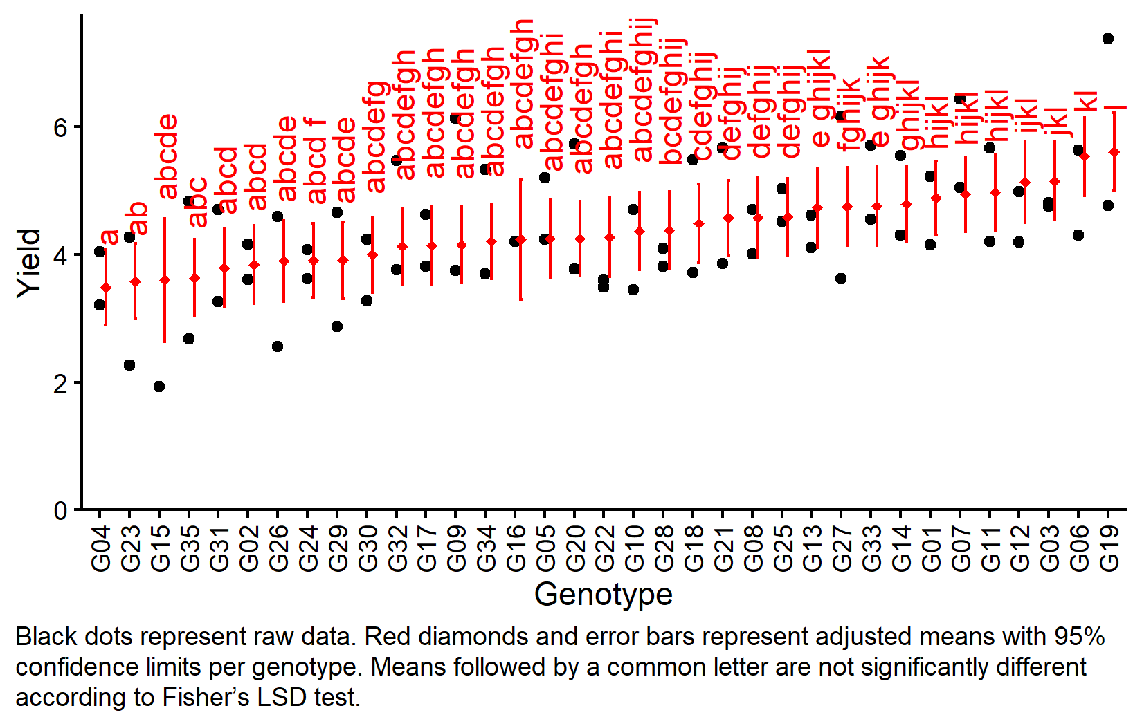

Bonus: Design Efficiency

Let’s assess the efficiency of the row-column design compared to a simple RCBD (ignoring the row and column structure):

# s.e.d. squared for RCBD (ignoring row/column structure)
avg_sed_rcbd <- lm(yield ~ gen + rep, data = dat) %>% 
  emmeans(pairwise ~ "gen", adjust = "none") %>%
  pluck("contrasts") %>%
  as_tibble() %>%
  pull("SE") %>%
  mean()

# Efficiency
avg_sed_rcbd^2 / sed_fixed^2

[1] 1.953932

An efficiency > 1 indicates that the row-column design is more efficient than a simple RCBD, meaning the row and column blocking successfully reduced experimental error.

Wrapping Up

You’ve now learned how to analyze data from a resolvable row-column design, which provides powerful control over two sources of spatial variation.

NoteKey Takeaways

1. Row-column designs control for two sources of variation simultaneously by blocking in both row and column directions within each replicate.

2. More flexible than Latin Square: Can accommodate any number of treatments, not limited to t×t arrangements.

3. Double blocking within replicates provides increased precision when spatial trends exist in two directions.

4. Model choice between fixed and random row/column effects can be based on which gives smaller average s.e.d.

5. The model with fixed effects: yield ~ gen + rep + rep:rowF + rep:colF (rows and columns nested within replicates).

6. Design efficiency > 1 compared to RCBD confirms the benefit of the additional row-column structure.

7. Missing data handling: Row-column designs can still be analyzed when some observations are missing, though precision may be affected.

Design Comparison Summary

Let’s summarize the progression of designs covered in this chapter series:

Design	Blocking Structure	Model Formula	Best For
CRD	None	y ~ trt	Homogeneous conditions
RCBD	Complete blocks	y ~ trt + block	One gradient
Latin Square	Rows + columns (complete)	y ~ trt + row + col	Two gradients, few treatments
Alpha Design	Incomplete blocks in reps	y ~ trt + rep + (1|rep:block)	Many treatments, one gradient
Augmented	Checks + entries	y ~ trt + block	Screening many unreplicated entries
Row-Column	Inc. rows + cols in reps	y ~ trt + rep + rep:row + rep:col	Many treatments, two gradients

References

Kempton, R. A., P. N. Fox, and M. Cerezo. 1997. Statistical Methods for Plant Variety Evaluation. Springer Netherlands. https://doi.org/10.1007/978-94-009-1503-9.