for (pkg in c("desplot", "emmeans", "ggtext", "here", "lme4",
              "lmerTest", "multcomp", "multcompView", "tidyverse")) {
  if (!require(pkg, character.only = TRUE)) install.packages(pkg)
}

library(desplot)
library(emmeans)
library(ggtext)
library(here)
library(lme4)
library(lmerTest)
library(multcomp)
library(multcompView)
library(tidyverse)To install and load all the packages used in this chapter, run the following code:
Augmented Designs
In the previous chapter, we analyzed an alpha design where all genotypes were replicated across blocks. However, in plant breeding and variety testing, we often face situations where we have many new genotypes to test but limited resources. Testing all genotypes with full replication may not be feasible.
What is an Augmented Design?
An augmented design (also called augmented block design) addresses this by including two types of entries:
- Check varieties (standards): Replicated across all blocks, providing a basis for estimating block effects
- New entries (test genotypes): Unreplicated, appearing in only one block each
The replicated checks allow us to estimate and adjust for block effects, which can then be applied to the unreplicated entries. This design maximizes the number of new entries that can be tested with limited resources while still allowing valid statistical comparisons.
The advantages of augmented designs include:
- Resource efficiency: Test many new entries without full replication
- Valid comparisons: Block effects estimated from checks are applied to all entries
- Flexibility: Can accommodate varying numbers of new entries per block
- Practical for screening: Ideal for early-stage variety trials with many candidates
The Trade-off
The key trade-off is precision: unreplicated entries have higher standard errors than replicated checks. This means comparisons involving new entries are less precise than comparisons between checks. However, for initial screening purposes, this is often acceptable.
Data
This example considers data published in Petersen (1994) from a yield trial laid out as an augmented design. The trial included 3 check varieties (st, ci, wa) replicated in all 6 blocks, and 30 new entries (numbered 1-30) each appearing in only one block.
Import
Rows: 48 Columns: 5
── Column specification ────────────────────────────────────────────────────────
Delimiter: ","
chr (2): gen, block
dbl (3): yield, row, col

ℹ Use `spec()` to retrieve the full column specification for this data.
ℹ Specify the column types or set `show_col_types = FALSE` to quiet this message.
# A tibble: 48 × 5
gen yield block row col
<chr> <dbl> <chr> <dbl> <dbl>
1 st 2972 I 1 1
2 14 2405 I 2 1
3 26 2855 I 3 1
4 ci 2592 I 4 1
5 17 2572 I 5 1
6 wa 2608 I 6 1
7 22 2705 I 7 1
8 13 2391 I 8 1
9 st 3122 II 1 2
10 ci 3023 II 2 2
# ℹ 38 more rowsThe dataset contains:
-
gen: Genotype identifier (3 checks: st, ci, wa; 30 new entries: 1-30) -
yield: Crop yield -
block: Six blocks (I-VI) -
rowandcol: Field plot coordinates for visualization
Format
Before analysis, we need to encode gen and block as factors:
# A tibble: 48 × 5
   gen   yield block   row   col
   <fct> <dbl> <fct> <dbl> <dbl>
 1 st     2972 I         1     1
 2 14     2405 I         2     1
 3 26     2855 I         3     1
 4 ci     2592 I         4     1
 5 17     2572 I         5     1
 6 wa     2608 I         6     1
 7 22     2705 I         7     1
 8 13     2391 I         8     1
 9 st     3122 II        1     2
10 ci     3023 II        2     2
# ℹ 38 more rows
Explore
Let’s first examine the summary statistics. Note the difference in replication between checks and new entries:
# A tibble: 33 × 4
   gen   count mean_yield sd_yield
   <fct> <int>      <dbl>    <dbl>
 1 st        6      2759.     832.
 2 ci        6      2726.     711.
 3 wa        6      2678.     615.
 4 19        1      3643       NA
 5 11        1      3380       NA
 6 07        1      3265       NA
 7 03        1      3055       NA
 8 04        1      3018       NA
 9 01        1      3013       NA
10 30        1      2955       NA
# ℹ 23 more rows
The three checks (ci, st, wa) each appear 6 times (once per block), while all new entries appear only once. This is the defining characteristic of an augmented design.
Now let’s look at the block structure:
# A tibble: 6 × 4
  block count mean_yield sd_yield
  <fct> <int>      <dbl>    <dbl>
1 VI        8      3205.     417.
2 II        8      2864.     258.
3 IV        8      2797.     445.
4 I         8      2638.     202.
5 III       8      2567.     440.
6 V         8      1390.     207.
We can see variation among blocks. Block II has the highest mean yield, while Block V has the lowest. Let’s visualize the data with different colors for checks and new entries:
# Define custom colors: greens for new entries, reds for checks
greens30 <- colorRampPalette(c("#bce2cc", "#00923f"))(30)
oranges3 <- colorRampPalette(c("#e4572e", "#ad0000"))(3)
gen_cols <- set_names(c(greens30, oranges3), nm = levels(dat$gen))ggplot(data = dat) +
aes(
y = yield,
x = gen,
color = gen,
shape = block
) +
geom_point() +
scale_x_discrete(
name = "Genotype"
) +
scale_y_continuous(
name = "Yield",
limits = c(0, NA),
expand = expansion(mult = c(0, 0.05))
) +
scale_color_manual(
guide = "none",
values = gen_cols
) +
scale_shape_discrete(
name = "Block"
) +
guides(shape = guide_legend(nrow = 1)) +
theme_classic() +
theme(
legend.position = "top",
axis.text.x = element_text(size = 7)
)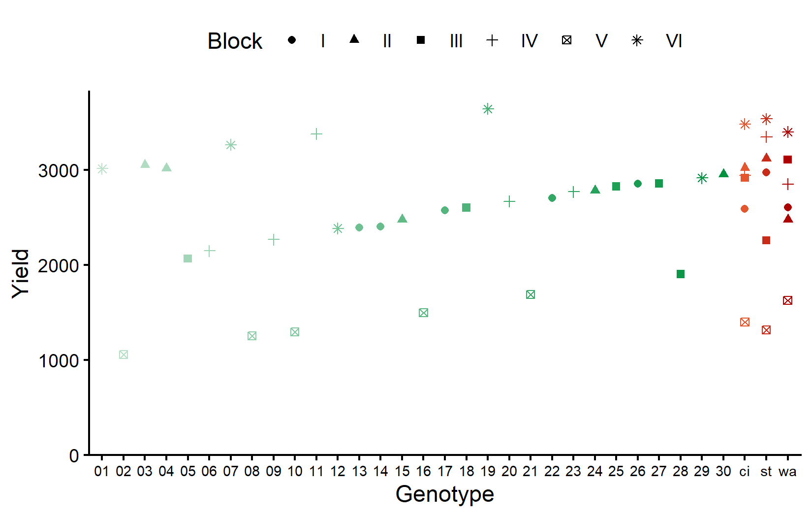
The checks (in red/orange on the right) show variation across blocks, allowing us to estimate block effects. Now let’s look at the field layout:
desplot(
  data = dat,
  flip = TRUE,
  form = gen ~ col + row, # fill color per genotype
  col.regions = gen_cols, # custom fill colors
  out1 = block, # line between blocks
  text = gen, # genotype names per plot
  cex = 1,
  shorten = FALSE,
  main = "Field layout",
  show.key = FALSE
) 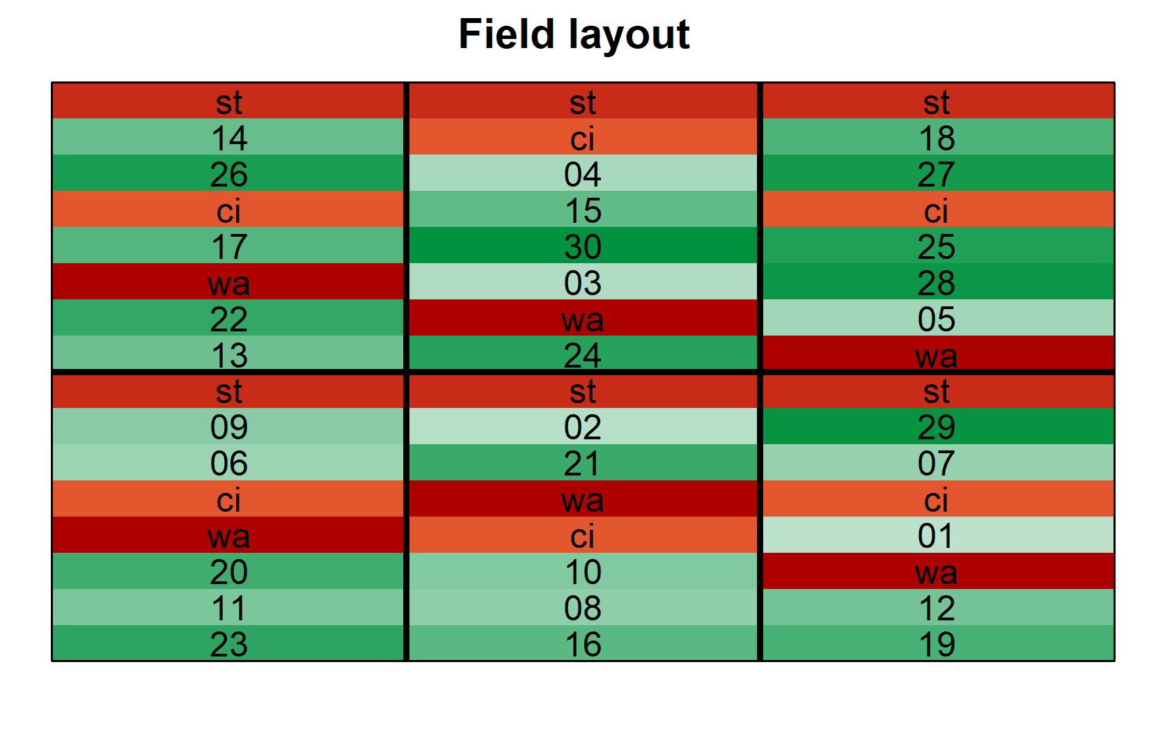
The layout shows how checks (st, ci, wa) are distributed across all blocks, while each new entry appears in only one block.
Model and ANOVA
Fixed Block Model
For an augmented design, we can fit the model with blocks as either fixed or random effects. Let’s start with fixed blocks:
mod_fb <- lm(yield ~ gen + block, data = dat)And compare with random blocks:
mod_rb <- lmer(yield ~ gen + (1 | block), data = dat)To determine which model is more appropriate for comparing genotypes, we compare the average standard error of a difference (s.e.d.):
# s.e.d. for fixed blocks model
sed_fixed <- mod_fb %>%
  emmeans(pairwise ~ "gen", adjust = "none") %>%
  pluck("contrasts") %>%
  as_tibble() %>%
  pull("SE") %>%
  mean()

# s.e.d. for random blocks model
sed_random <- mod_rb %>%
  emmeans(pairwise ~ "gen", adjust = "none", lmer.df = "kenward-roger") %>%
  pluck("contrasts") %>%
  as_tibble() %>%
  pull("SE") %>%
  mean()

tibble(
  model = c("Fixed blocks", "Random blocks"),
  mean_sed = c(sed_fixed, sed_random)
)
# A tibble: 2 × 2
model mean_sed
<chr> <dbl>
1 Fixed blocks 461.
2 Random blocks 462.In this case, the fixed blocks model has a slightly smaller s.e.d., so we’ll use it for our analysis.
WarningModel assumptions met?
It is at this point (i.e. after fitting the model and before interpreting the ANOVA) that one should check whether the model assumptions are met. Find out more in Appendix A1: Model Diagnostics.
Conducting the ANOVA
ANOVA <- anova(mod_fb)
ANOVA
Analysis of Variance Table
Response: yield
Df Sum Sq Mean Sq F value Pr(>F)
gen 32 12626173 394568 4.331 0.0091056 **
block 5 6968486 1393697 15.298 0.0002082 ***
Residuals 10 911027 91103
---
Signif. codes: 0 '***' 0.001 '**' 0.01 '*' 0.05 '.' 0.1 ' ' 1The genotype effect is statistically significant (p < 0.05), indicating differences among genotypes. The block effect is also significant, confirming that blocking was beneficial.
Mean Comparisons
 gen emmean  SE df lower.CL upper.CL .group
 12    1632 341 10      164     3100  a
 06    1823 341 10      355     3291  a
 28    1862 341 10      394     3330  a
 09    1943 341 10      475     3411  a
 05    2024 341 10      556     3492  a
 29    2162 341 10      694     3630  a
 01    2260 341 10      792     3728  a
 15    2324 341 10      856     3792  a
 02    2330 341 10      862     3798  a
 20    2345 341 10      877     3813  a
 13    2388 341 10      920     3856  a
 14    2402 341 10      934     3870  a
 23    2445 341 10      977     3913  a
 07    2512 341 10     1044     3980  a
 08    2528 341 10     1060     3996  a
 18    2562 341 10     1094     4030  a
 10    2568 341 10     1100     4036  a
 17    2569 341 10     1101     4037  a
 24    2630 341 10     1162     4098  a
 wa    2678 123 10     2148     3208  a
 22    2702 341 10     1234     4170  a
 ci    2726 123 10     2195     3256  a
 st    2759 123 10     2229     3289  a
 16    2770 341 10     1302     4238  a
 25    2784 341 10     1316     4252  a
 30    2802 341 10     1334     4270  a
 27    2816 341 10     1348     4284  a
 26    2852 341 10     1384     4320  a
 04    2865 341 10     1397     4333  a
 19    2890 341 10     1422     4358  a
 03    2902 341 10     1434     4370  a
 21    2963 341 10     1495     4431  a
 11    3055 341 10     1587     4523  a

Results are averaged over the levels of: block
Confidence level used: 0.95
Conf-level adjustment: sidak method for 33 estimates
P value adjustment: tukey method for comparing a family of 33 estimates
significance level used: alpha = 0.05
NOTE: If two or more means share the same grouping symbol,
      then we cannot show them to be different.
      But we also did not show them to be the same.
Notice that while some genotypes have higher adjusted means than others, no significant differences are detected with Tukey adjustment. This is partly because unreplicated entries have large confidence intervals. For example, genotype 11 has the highest adjusted mean (3055) but its confidence interval is wide.
Visualizing Results
my_caption <- "Dots represent raw data (green = new entries, red = checks). Red diamonds and error bars represent adjusted means with 95% confidence limits per genotype. Means followed by a common letter are not significantly different according to the Tukey test."

ggplot() +
  aes(x = gen) +
  # colored dots representing the raw data
  geom_point(
    data = dat,
    aes(y = yield, color = gen)
  ) +
  # red diamonds representing the adjusted means
  geom_point(
    data = mean_comp,
    aes(y = emmean),
    shape = 18,
    color = "red",
    position = position_nudge(x = 0.2)
  ) +
  # red error bars representing the confidence limits of the adjusted means
  geom_errorbar(
    data = mean_comp,
    aes(ymin = lower.CL, ymax = upper.CL),
    color = "red",
    width = 0.1,
    position = position_nudge(x = 0.2)
  ) +
  # red letters
  geom_text(
    data = mean_comp,
    aes(y = upper.CL, label = str_trim(.group)),
    color = "red",
    vjust = -0.2,
    position = position_nudge(x = 0.2)
  ) +
  scale_color_manual(
    guide = "none",
    values = gen_cols
  ) +
  scale_x_discrete(
    name = "Genotype",
    limits = as.character(mean_comp$gen)
  ) +
  scale_y_continuous(
    name = "Yield",
    limits = c(0, NA),
    expand = expansion(mult = c(0, 0.1))
  ) +
  labs(caption = my_caption) +
  theme_classic() +
  theme(plot.caption = element_textbox_simple(margin = margin(t = 5)),
        plot.caption.position = "plot",
        axis.text.x = element_text(size = 7))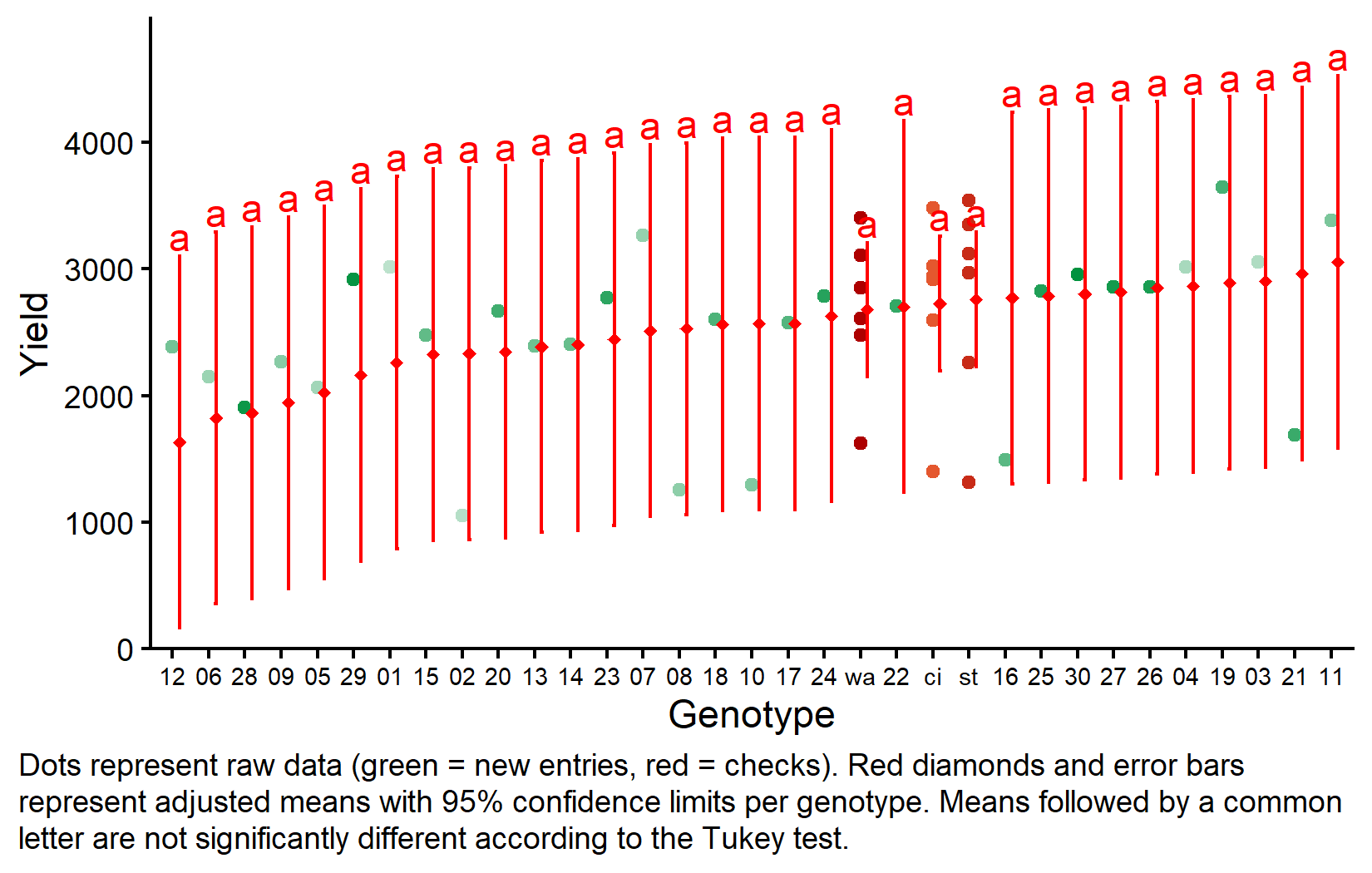
The plot clearly shows the difference in precision: checks (on the right) have much narrower confidence intervals due to replication, while new entries have wide intervals based on single observations adjusted for block effects.
Bonus: Variance Components
We can extract variance components from both models to understand the sources of variation:
# A tibble: 1 × 2
  source                 variance
  <chr>                     <dbl>
1 Residual (fixed model)   91103.
# A tibble: 2 × 2
grp variance
<chr> <dbl>
1 block 434198.
2 Residual 91103.Wrapping Up
You’ve now learned how to analyze data from an augmented design, which is particularly useful for screening many new entries with limited resources.
NoteKey Takeaways
Augmented designs include replicated checks and unreplicated new entries, maximizing the number of entries that can be tested.
Checks estimate block effects which are then applied to adjust all entries, including unreplicated ones.
The trade-off is precision: Unreplicated entries have wider confidence intervals than replicated checks.
Model choice (fixed vs. random blocks) can be based on which gives smaller average s.e.d. for genotype comparisons.
Practical application: Augmented designs are ideal for early-stage screening trials where many candidates need initial evaluation.
Interpretation caution: Lack of significant differences doesn’t mean entries are equal - it may reflect low power for unreplicated comparisons.
References
Petersen, Roger G. 1994. Agricultural Field Experiments. CRC Press. https://doi.org/10.1201/9781482277371.
Citation
BibTeX citation:
@online{schmidt2026,
  author = {{Dr. Paul Schmidt}},
  publisher = {BioMath GmbH},
  title = {5. {One-way} {ANOVA} in an {Augmented} {Design}},
  date = {2026-03-04},
  url = {https://biomathcontent.netlify.app/content/lin_mod_exp/05_oneway_augmented.html},
  langid = {en}
}
For attribution, please cite this work as:
Dr. Paul Schmidt. 2026. “5. One-Way ANOVA in an Augmented
Design.” BioMath GmbH. March 4, 2026. https://biomathcontent.netlify.app/content/lin_mod_exp/05_oneway_augmented.html.