To install and load all the packages used in this chapter, run the following code:
Statistical models make assumptions about the data, and results can be misleading if these assumptions are severely violated. This chapter covers how to check whether the assumptions of a linear model are reasonably met — a process known as model diagnostics. We start with a quick, practical approach and then progressively go deeper for those who want more detail.
The Quick Version
You fitted a linear model and you just want the ANOVA results — but somewhere in a lecture or a textbook, someone told you to “check model assumptions” first. Fair enough. Here is the fastest way to do it so you can move on with confidence. We use the built-in PlantGrowth dataset as an example throughout this chapter:
mod <- lm(weight ~ group, data = PlantGrowth)Note that both the PlantGrowth data and the lm() function come with base R and thus don’t need any extra packages. Now create the standard diagnostic plots:
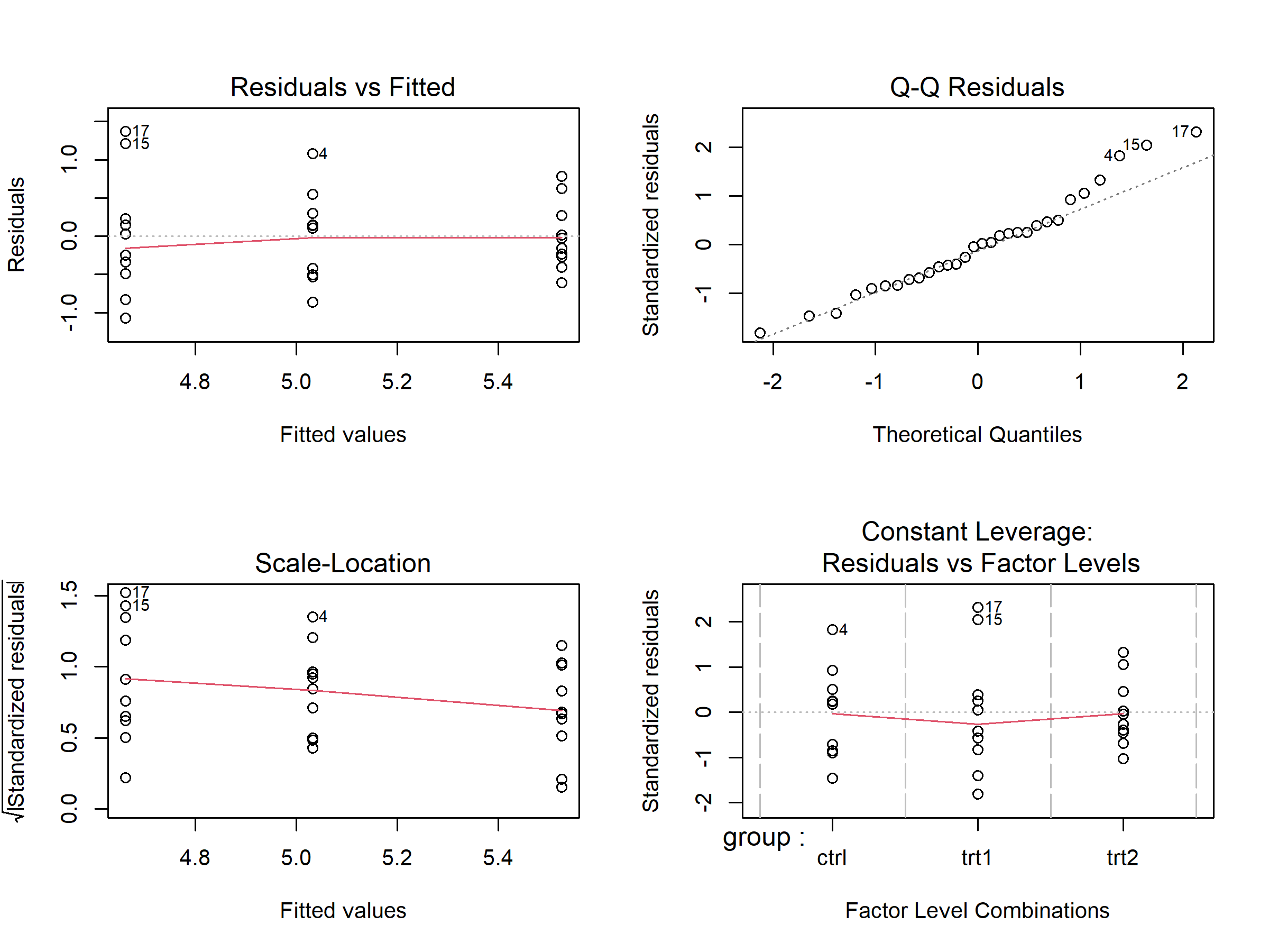
The par(mfrow = ...) lines1 are not part of the diagnostics — plot(mod) is the key command. These four plots give you a quick overview:
| Plot | What to check | What’s OK |
|---|---|---|
| Residuals vs Fitted (top-left) | Random scatter around zero? | No obvious curves or funnel shapes |
| Q-Q Residuals (top-right) | Dots close to the diagonal line? | Most points follow the line |
| Scale-Location (bottom-left) | Roughly even spread? | No clear funnel or trend |
| Residuals vs Factor Levels (bottom-right) | Any extreme outliers? | No points far beyond Cook’s distance lines |
If the plots look roughly OK — no dramatic patterns, no extreme outliers — you can proceed with your analysis. Linear models are quite robust to minor deviations from perfect assumptions. If something looks clearly problematic, read the sections below for guidance on what to do.
The {easystats} Alternative
If you want a more comprehensive set of diagnostic plots in a single call, the {easystats} package (which we already loaded above) provides check_model():
check_model(mod)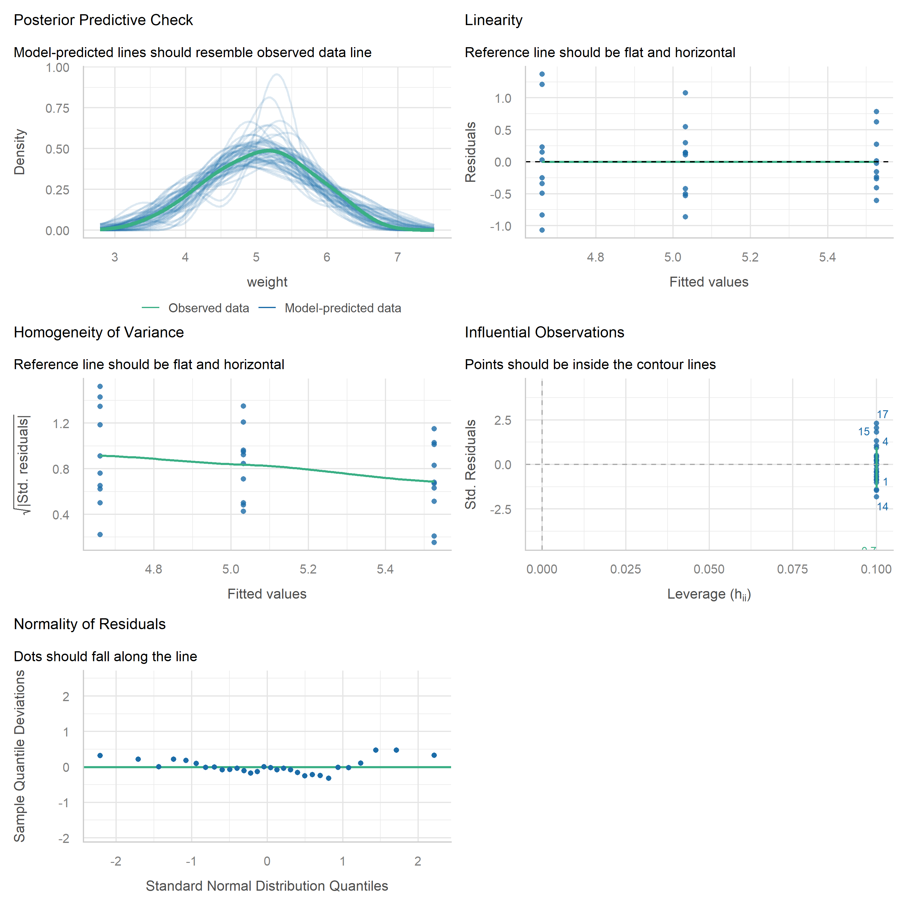
This produces a multi-panel figure that covers the key assumptions — including checks for normality, homoscedasticity, influential observations, and collinearity — all at once. It is a great way to get a quick yet thorough overview, and the plots are arguably easier to read than the base R versions. Either approach works well for routine diagnostics.
Understanding the Assumptions
Linear models (including ANOVA) rely on several assumptions. Let’s go through each one and understand what to look for.
Independence
Assumption: Individual observations are independent of each other.
This assumption cannot be checked with diagnostic plots or statistical tests. Instead, it must be ensured through proper experimental design and randomization. If your experiment was properly randomized (as it should be in any well-designed study), this assumption is typically met.
When independence is violated — for example in repeated measures over time, spatially correlated field experiments, or hierarchical data structures — standard errors become unreliable. In such cases, specialized methods like mixed-effects models should be used instead.
Normality of Residuals
Assumption: The model residuals follow a normal distribution.
A very common mistake is to check whether the raw response variable (e.g. yield) is normally distributed. This is not what the assumption is about. What needs to be approximately normal are the model’s residuals — i.e. the deviations between observed and fitted values. See Kozak and Piepho (2018) (section “4 | Answering Question 1”) for details.
The QQ plot (quantile-quantile plot) is the primary tool for assessing normality. It plots the residuals against what they would look like if they were perfectly normal. If normality holds, the points fall along the diagonal line:
plot(mod, which = 2)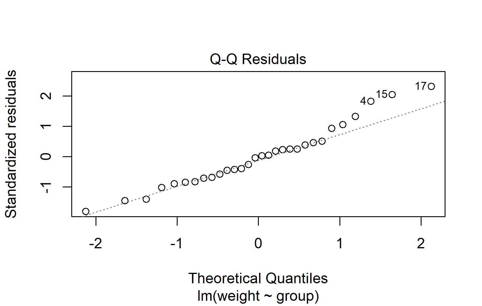
When interpreting QQ plots, focus on the overall pattern rather than individual points:
- Good normality: Points follow the diagonal line closely, with perhaps minor deviations at the very ends.
- Heavy tails: Points curve away from the line at both ends (S-shape).
- Skewness: Points systematically deviate from the line in one direction.
- Outliers: One or two points far from the line, while the rest follow it well.
Don’t worry about minor deviations in QQ plots. Linear models handle mild non-normality well, especially when sample sizes are adequate (roughly n > 15 per group). The Central Limit Theorem ensures that even with non-normal residuals, the ANOVA F-test remains approximately valid for moderate to large samples.
Homoscedasticity
Assumption: The error variance is constant across all groups / fitted values.
Also referred to as homoscedasticity (the opposite of heteroscedasticity). The residuals-vs-fitted plot helps assess this assumption. The residuals should form an approximately even horizontal band around zero:
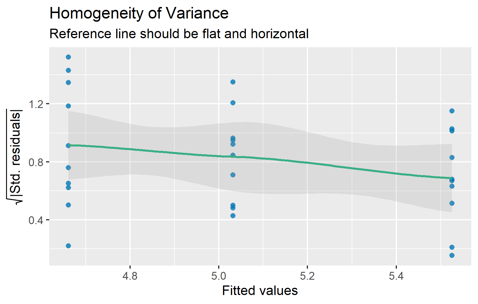
If the spread of residuals clearly increases or decreases with the fitted values (a “funnel” shape), variance homogeneity may be violated. Minor differences in spread across groups are usually not problematic — ANOVA is fairly robust when the ratio of the largest to smallest group variance is less than about 3:1.
Linearity
Assumption: The response can be written as a linear combination of the predictors.
This assumption is also checked via the residuals-vs-fitted plot (the top-left panel from the four-panel plot above). At any fitted value, the mean of the residuals should be roughly zero. If there is a clear curved pattern rather than a random scatter, the linearity assumption may not hold.
Note that for models with only categorical predictors (like all the ANOVA examples in this course), linearity is automatically satisfied — the model simply estimates a separate mean for each group. The curved patterns shown below can only arise when a continuous predictor is involved (e.g. in regression). Still, understanding these patterns is useful because many real-world analyses combine categorical and continuous predictors.
To illustrate what problematic patterns look like compared to a healthy residual pattern, here are three simulated examples:
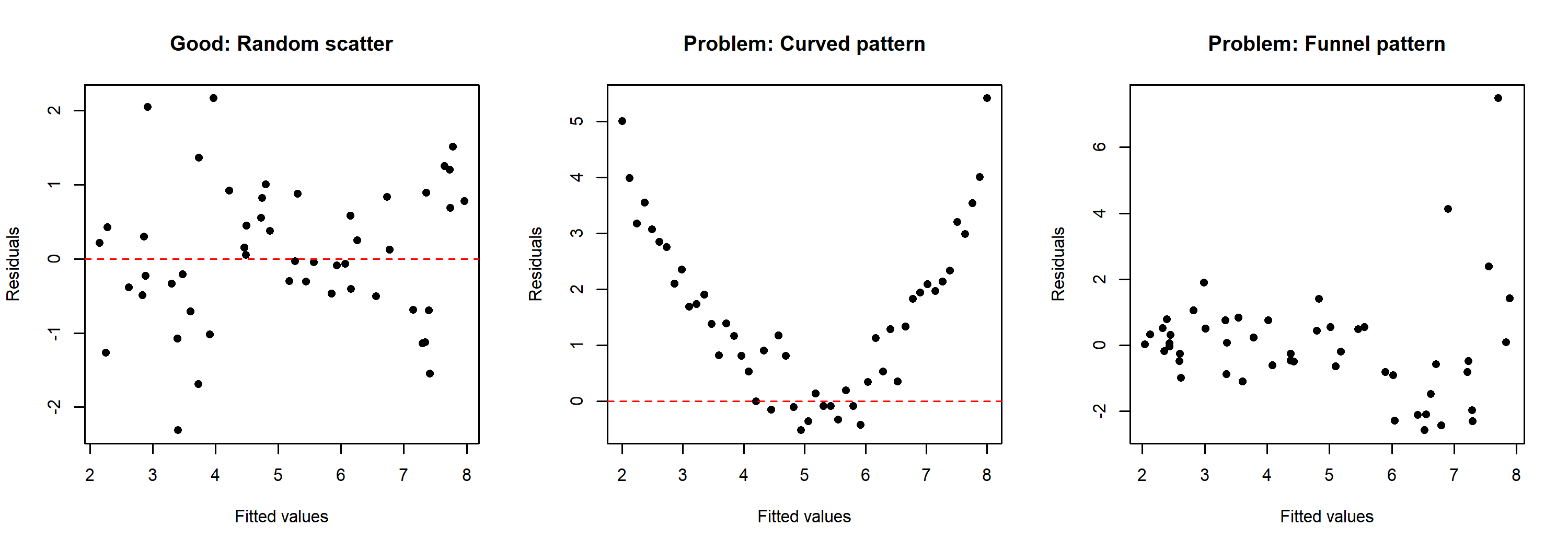
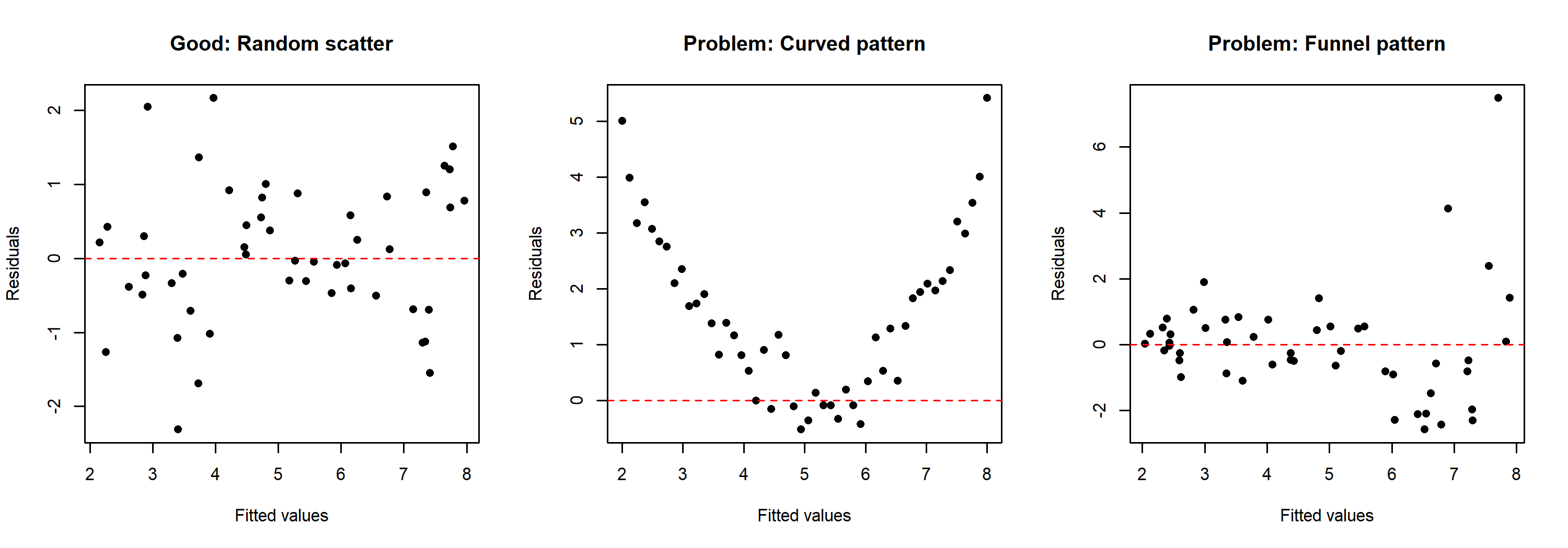
The left panel shows a well-behaved residual pattern with random scatter around zero. The center panel shows a curved pattern, suggesting that the relationship between predictor and response is not linear. The right panel shows a funnel pattern where the spread of residuals increases with fitted values — this indicates heteroscedasticity rather than a linearity problem.
Going Deeper
The sections above cover what is needed for routine model diagnostics. What follows goes beyond the basics and addresses more nuanced questions: Why are diagnostic tests problematic? How can influential observations be identified? And what can be done when assumptions are clearly violated?
Why Plots Instead of Tests?
It might seem natural to use a statistical test (like the Shapiro-Wilk test for normality) to “objectively” check assumptions. However, there is growing consensus among statisticians that diagnostic plots are more informative than statistical tests for this purpose.
Kozak and Piepho (2018) provide a clear argument for why this is the case:
According to many authors (e.g., Atkinson, 1987; Belsley, Kuh, & Welsch, 2005; Kozak, 2009; Moser & Stevens, 1992; Quinn & Keough, 2002; Rasch, Kubinger, & Moder, 2011; Schucany & Ng, 2006), significance tests should not be used for checking assumptions. Diagnostic residual plots are a better choice.
[…]
There are two possible reasons for the overuse of statistical tests to check assumptions. First, many researchers base their knowledge on books first published 40 years ago or earlier. Back then, using statistical tests was relatively simple while using diagnostic plots was difficult; thus, these books advised the former, often even not mentioning the latter. Second, most statistical software offers statistical tests for checking assumptions as a default. Using default tests is simple, so users use them. However, we explained why we think that significance tests are not a good way of checking assumptions (in general, not only for ANOVA). First of all, with large samples (a very desirable situation) we risk that even small (and irrelevant) departures from the null hypothesis (which states that the assumption is met) will be detected as significant, and so we would need to reject the hypothesis and state that the assumption is not met. With small samples, the situation is opposite: much larger (and important) departures would not be found significant. Thus, our advice is to use diagnostic plots instead of hypothesis testing to check ANOVA assumptions.
To see this problem in action, consider the normality tests for our example model:
ols_test_normality(mod)-----------------------------------------------
Test Statistic pvalue
-----------------------------------------------
Shapiro-Wilk 0.9661 0.4379
Kolmogorov-Smirnov 0.1101 0.8215
Cramer-von Mises 3.6109 0.0000
Anderson-Darling 0.3582 0.4299
-----------------------------------------------The QQ plot above looks perfectly fine, yet the tests do not all agree — notice how individual tests can flag a “significant” deviation even when the visual impression is clearly acceptable. This contradictory situation illustrates exactly why relying on tests rather than visual inspection can be misleading.
For completeness, here are common tests for variance homogeneity:
# Breusch-Pagan test
ols_test_breusch_pagan(mod)
 Breusch Pagan Test for Heteroskedasticity
 -----------------------------------------
 Ho: the variance is constant
 Ha: the variance is not constant

               Data
 ----------------------------------
 Response : weight
 Variables: fitted values of weight

        Test Summary
 -----------------------------
 DF            =    1
 Chi2          =    3.000303
 Prob > Chi2   =    0.08324896
# Bartlett test (designed for comparing group variances)
bartlett.test(weight ~ group, data = PlantGrowth)
    Bartlett test of homogeneity of variances

data:  weight by group
Bartlett's K-squared = 2.8786, df = 2, p-value = 0.2371
Both are non-significant (p > 0.05), which is consistent with the diagnostic plots. But remember: a non-significant test does not guarantee the assumption is met — it may simply reflect insufficient statistical power.
Outliers and Influential Observations
Sometimes individual observations have a disproportionate influence on the model results. These are not necessarily wrong data points, but it is important to be aware of them.
Cook’s Distance quantifies how much all fitted values change when a single observation is removed. A common rule of thumb: observations with Cook’s distance greater than 4/n deserve a closer look:
plot(mod, which = 4)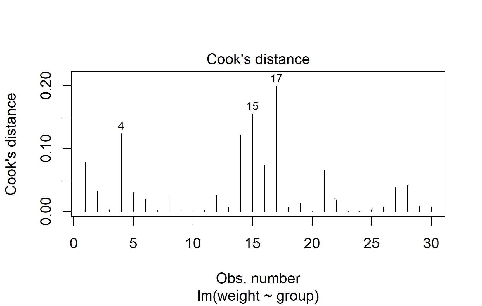
In our example, observations 15 and 17 have the highest Cook’s distance. With the threshold at 4/30 ≈ 0.13, these two values are just slightly above it. This is quite mild — Cook’s distance values greater than 1.0 would indicate a strong concern.
DFBETAS measure how much each regression coefficient changes when a single observation is removed. Observations with |DFBETAS| > 2/√n warrant attention. It is important to check DFBETAS for all model coefficients, not just the intercept — an observation might strongly affect a group contrast without changing the overall mean:
n <- nrow(PlantGrowth)
db <- dfbetas(mod)

data.frame(
  obs = 1:n,
  cooks_d = round(cooks.distance(mod), 4),
  dfb_intercept = round(db[, 1], 4),
  dfb_grouptrt1 = round(db[, 2], 4),
  dfb_grouptrt2 = round(db[, 3], 4)
) %>%
  filter(
    cooks_d > 4 / n |
    if_any(starts_with("dfb_"), \(x) abs(x) > 2 / sqrt(n))
  )
obs cooks_d dfb_intercept dfb_grouptrt1 dfb_grouptrt2
1 1 0.0787 -0.4967 0.3512 0.3512
4 4 0.1231 0.6367 -0.4502 -0.4502
14 14 0.1215 0.0000 -0.4469 0.0000
15 15 0.1548 0.0000 0.5143 0.0000
17 17 0.1985 0.0000 0.5981 0.0000In practice, when influential observations are identified, the most useful approach is to run the analysis both with and without them and compare the conclusions. If they agree, there is no cause for concern.
What to Do When Assumptions Are Violated
When diagnostic plots reveal clear problems, there are several options depending on the nature and severity of the violation.
Data Transformation
Transforming the response variable with a mathematical function (e.g. square root or logarithm) can often improve model diagnostics substantially. Here is an example using data from a cucumber trial in a Latin Square Design (the same data as in Chapter 3):
We fit two models — one with the original response and one with the square-root-transformed response — and compare their QQ plots side by side:
The QQ plot for the square root model is clearly closer to the diagonal line, so we proceed with the ANOVA on the transformed scale:
anova(mod_sqrt)Analysis of Variance Table
Response: sqrt(yield)
Df Sum Sq Mean Sq F value Pr(>F)
gen 3 10.5123 3.5041 8.8966 0.01256 *
rowF 3 5.0283 1.6761 4.2555 0.06228 .
colF 3 4.2121 1.4040 3.5647 0.08670 .
Residuals 6 2.3632 0.3939
---
Signif. codes: 0 '***' 0.001 '**' 0.01 '*' 0.05 '.' 0.1 ' ' 1The ANOVA shows a significant effect of genotype. For mean comparisons via post hoc tests, the means can be presented on the backtransformed (= original) scale, as long as it is made clear to the reader that the model fit and mean comparisons were performed on the square root scale:
Note: adjust = "tukey" was changed to "sidak"
because "tukey" is only appropriate for one set of pairwise comparisons
gen response SE df lower.CL upper.CL .group
Poinsett 20.9 2.87 6 12.0 32.1 a
Sprint 25.1 3.14 6 15.3 37.3 a
Guardian 30.4 3.46 6 19.5 43.7 ab
Dasher 45.3 4.23 6 31.7 61.4 b
Results are averaged over the levels of: rowF, colF
Confidence level used: 0.95
Conf-level adjustment: sidak method for 4 estimates
Intervals are back-transformed from the sqrt scale
Note: contrasts are still on the sqrt scale. Consider using
regrid() if you want contrasts of back-transformed estimates.
P value adjustment: tukey method for comparing a family of 4 estimates
significance level used: alpha = 0.05
NOTE: If two or more means share the same grouping symbol,
then we cannot show them to be different.
But we also did not show them to be the same. Note that type = "response" performs the backtransformation automatically. This only works when the transformation is specified inside the model formula (as we did with sqrt(yield) in lm()), not when a transformed column is created beforehand.
Alternative Methods (and Their Limitations)
When assumptions are violated and transformation does not help, several alternative methods exist. We briefly introduce them here, but with an important caveat: most of these alternatives only work for the simplest experimental designs.
Welch’s ANOVA does not assume equal variances across groups:
# Welch's ANOVA (does not assume equal variances)
oneway.test(weight ~ group, data = PlantGrowth, var.equal = FALSE)
    One-way analysis of means (not assuming equal variances)

data:  weight and group
F = 5.181, num df = 2.000, denom df = 17.128, p-value = 0.01739
Robust standard errors keep the original model but adjust the standard errors to account for heteroscedasticity:
for (pkg in c("lmtest", "sandwich")) {
  if (!require(pkg, character.only = TRUE)) install.packages(pkg)
}
t test of coefficients:

            Estimate Std. Error t value Pr(>|t|)
(Intercept)  5.03200    0.19436 25.8896  < 2e-16 ***
grouptrt1   -0.37100    0.32828 -1.1301  0.26836
grouptrt2    0.49400    0.24401  2.0245  0.05291 .
---
Signif. codes:  0 '***' 0.001 '**' 0.01 '*' 0.05 '.' 0.1 ' ' 1
Non-parametric tests like the Kruskal-Wallis test relax the normality assumption by working with ranks instead of raw values:
kruskal.test(weight ~ group, data = PlantGrowth)
    Kruskal-Wallis rank sum test

data:  weight by group
Kruskal-Wallis chi-squared = 7.9882, df = 2, p-value = 0.01842
Note that Kruskal-Wallis is not entirely “assumption-free” — it still assumes that the distributions in each group have the same shape, just possibly shifted in location.
All three methods shown above work well for the simple one-way case demonstrated here. However, most real-world experiments involve multiple treatment factors, blocking structures, or random effects — and that is where these alternatives reach their limits:
- Welch’s ANOVA only handles one-way designs. There is no Welch version for two-way ANOVA, split-plot designs, or models with block effects.
- Robust standard errors can be applied more broadly, but standard implementations do not extend cleanly to mixed-effects models or complex variance structures.
- Non-parametric tests exist for a few simple designs — Kruskal-Wallis for one-way layouts, the Friedman test for RCBD — but there are no straightforward non-parametric equivalents for factorial designs, incomplete block designs, or split-plot experiments.
In practice, this means that for most of the experimental designs covered in this course (Latin Square, Alpha Design, Row-Column, etc.), these alternatives are usually not available. The realistic options when assumptions are violated in complex designs are: (1) data transformation, (2) using generalized linear models (GLMs — see the outlook below), or (3) accepting that mild violations are not a problem (see the robustness discussion below).
How Robust Are Linear Models?
Linear models are more robust to assumption violations than is commonly taught. Research has consistently shown that:
- ANOVA is robust to moderate violations of both normality and variance homogeneity, especially when sample sizes are balanced and adequate.
- The Central Limit Theorem ensures that even with non-normal residuals, test statistics converge to their expected distributions as sample sizes grow.
- Minor violations are the norm, not the exception. Most real-world data deviate from perfect assumptions to some degree.
As a rough guideline:
| Sample size per group | Practical advice |
|---|---|
| Small (n < 15) | Assumption violations are more impactful. Consider exact tests or robust methods. Interpret diagnostics carefully. |
| Moderate (15–50) | Standard ANOVA is usually robust to mild violations. Focus on detecting severe problems only. |
| Large (50+) | Central Limit Theorem provides strong protection. Assumption checking is less critical, but diagnostic plots can still reveal data quality issues. |
The key message is: do not discard your ANOVA results because of minor imperfections in diagnostic plots. Focus on clear, unambiguous violations. When in doubt, run the analysis both with the standard approach and a robust alternative — if the conclusions agree, the assumption violation was not consequential.
General
- What’s normal anyway? Residual plots are more telling than significance tests when checking ANOVA assumptions (Kozak and Piepho 2018)
- Chapter 13 Model Diagnostics in Applied Statistics with R (Dalpiaz, 2022)
- {olsrr} R package documentation
Normality
- For this specific purpose, QQ plots may also be called Normal probability plots
Variance Homogeneity
Transformation
- Chapter 3.3 in Dormann and Kühn (2011)
Outlook: Generalized Linear Models
So far, this chapter has dealt with situations where the assumptions of a linear model are approximately met or where mild violations can be tolerated. But what about data that fundamentally cannot meet these assumptions?
Consider count data (e.g. number of insects per plant) or proportions (e.g. percentage of germinated seeds). These response variables are inherently non-normal: counts are discrete and cannot be negative, proportions are bounded between 0 and 1. Transformations (like log for counts or arcsine-square-root for proportions) have been used for decades and can help, but they do not fully resolve the fundamental mismatch between the data and the normal distribution. Trying to force such data into a standard linear model often leads to persistent diagnostic problems — and that is a sign that the model itself may be the wrong tool for the job.
Generalized Linear Models (GLMs) solve this by extending the linear model framework to handle different types of response variables directly. Instead of assuming normally distributed residuals, a GLM lets you specify a distribution that matches the nature of your data:
| Data type | Distribution | Example |
|---|---|---|
| Counts (0, 1, 2, …) | Poisson | Number of insects per plot |
| Binary outcomes (yes/no) | Binomial | Germinated or not |
| Proportions (0–1) | Beta or Binomial | Infection rate |
| Positive continuous data | Gamma | Yield with right skew |
The beauty of GLMs is that the model assumptions are built around the actual data-generating process rather than forcing the data into a normal framework. This means that when your diagnostic plots show systematic problems that transformation cannot fix, the answer is often not “try harder to meet the assumptions” but rather “use a model whose assumptions match your data.”
GLMs use the same R syntax you already know — glm() instead of lm() — and they integrate with the same tools for ANOVA-type analysis (anova(), emmeans()), blocking structures, and factorial designs. A detailed treatment of GLMs is beyond the scope of this chapter, but it is good to know that they exist as a principled solution for data that do not fit the linear model framework.
Start with
plot(mod)— the four-panel diagnostic plot provides a quick visual check of the key assumptions. Alternatively, usecheck_model(mod)from {easystats} for a more comprehensive overview.Use plots, not tests for checking assumptions. Statistical tests for normality or variance homogeneity often mislead, especially with small or large samples.
Check residuals, not raw data. Normality must be assessed on the model residuals, not the response variable.
Minor violations are usually not a problem. Linear models are robust, especially with adequate sample sizes.
When violations are severe, data transformation is usually the first and most broadly applicable remedy.
Alternative methods have limits. Welch’s ANOVA, robust standard errors, and non-parametric tests only work for the simplest designs. For complex experiments, consider transformation or GLMs.
Report transparently. Document your diagnostic process and any actions taken.
References
Footnotes
par(mfrow = c(2, 2))is an R base graphics command that arranges the next plots in a 2-by-2 grid. It has nothing to do with model diagnostics — it simply tells R to display four plots at once instead of one at a time. Thepar(mfrow = c(1, 1))at the end resets this back to the default single-plot layout.↩︎
Citation
@online{schmidt2026,
  author = {{Dr. Paul Schmidt}},
  title = {A1. {Model} {Diagnostics}},
  date = {2026-03-04},
  url = {https://biomathcontent.netlify.app/content/lin_mod_exp/a1_modeldiagnostics.html},
  langid = {en}
}