4. Export and Canvas

for (pkg in c("ggplot2")) {
  if (!require(pkg, character.only = TRUE)) install.packages(pkg)
}

In the previous chapters we built plots that looked great in the RStudio preview panel. But the preview is deceptive: it adjusts every plot to the current window size, so fonts, line widths, and spacing change whenever the window is resized. A plot that looks balanced in a wide window may have oversized text in a narrow one - or vice versa. For reproducible, publication-ready output, one needs to export at a fixed size and resolution.

This chapter covers two tools for this: ggsave() for direct file export, and the {camcorder} package for a WYSIWYG preview workflow. Both solve the same fundamental problem - the canvas problem.

The canvas problem

To understand why export dimensions matter, consider the following demonstration. We create a simple PlantGrowth plot and render it at two very different canvas sizes:

p <- ggplot(PlantGrowth, aes(x = group, y = weight)) +
  geom_point() +
  labs(title = "Plant Growth Experiment") +
  theme_minimal()

At a very small canvas (3 x 1 inches), text elements dominate the plot and the data is barely visible:

p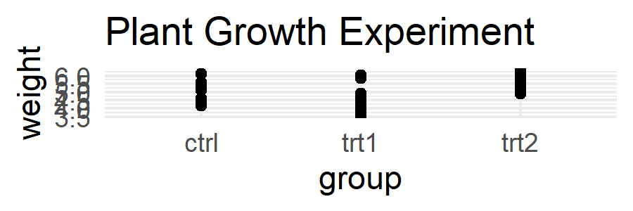

At a larger canvas (8 x 6 inches), the same plot has plenty of breathing room but the text appears proportionally tiny:

p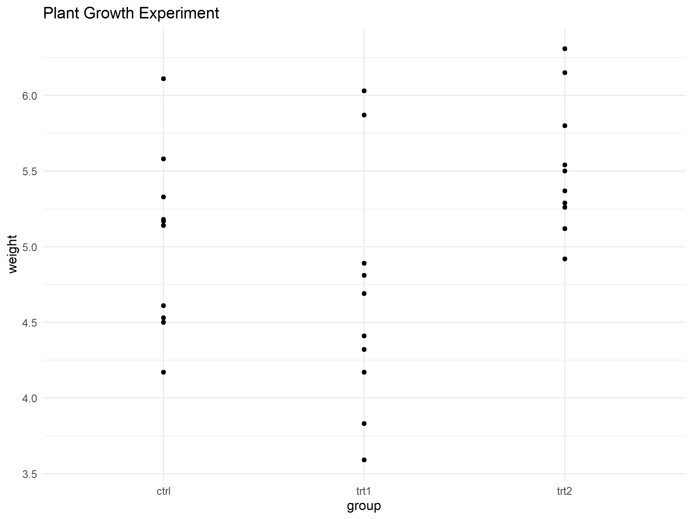

The code is identical - only the canvas size changed. This is the core insight: text and geom sizes in ggplot2 are absolute (measured in points or millimeters), while the canvas is relative. A 12pt title takes the same physical space regardless of whether the plot is 3 inches or 8 inches wide. On a small canvas, 12pt text fills most of the area; on a large canvas, it looks like a footnote.

This means that the “right” font size, line width, and point size all depend on the export dimensions. A plot designed for a full-page journal figure (7 x 5 inches) will look wrong in a presentation slide (10 x 5.6 inches) - and both will look wrong in the RStudio preview panel, which has neither dimension.

ImportantThe preview is not the output

The RStudio/Positron Plots panel rescales every plot to the current window size. This is convenient for exploration but misleading for final output. Always check the exported file (PNG, PDF, etc.) rather than the preview.

ggsave

The ggsave() function exports a ggplot to a file with full control over dimensions and resolution:

ggsave(
  filename = "my_plot.png",
  plot = p,
  width = 6,
  height = 4,
  units = "in",
  dpi = 300
)

The key arguments are:

• filename: Output path. The file extension determines the format (.png, .pdf, .svg, .jpg, etc.)
• plot: The ggplot object. If omitted, ggsave() saves the last plot displayed
• width and height: Canvas dimensions
• units: "in" (inches), "cm", "mm", or "px"
• dpi: Resolution in dots per inch. 300 is standard for print, 150 for screen, 72 for quick previews
• scale: Multiplier applied to the canvas size. scale = 2 doubles all dimensions, effectively halving the relative size of text and points

TipCommon export sizes

Some typical dimension combinations:

Use case	Width	Height	DPI
Journal figure (single column)	3.5 in	3 in	300
Journal figure (full width)	7 in	5 in	300
Presentation slide (16:9)	10 in	5.6 in	150
Poster panel	8 in	6 in	300
Web/blog	8 in	5 in	150

A common workflow is to iterate: export, open the file, check if text sizes and spacing look right, adjust width/height or theme(base_size = ...), export again. This loop is effective but tedious - which is where camcorder helps.

TipSpeeding up the export-check loop

Two tricks make the iterate-and-check cycle faster:

1. Open the file directly from R with shell.exec("my_plot.png") (Windows) or browseURL("my_plot.png") (cross-platform). This saves the manual step of navigating to the file in a file manager.
2. Export to PDF during development and open it in a viewer that does not lock the file. Sumatra PDF (Windows, free) reloads the file automatically whenever it changes on disk - one can re-run ggsave() and see the updated plot instantly without closing and reopening. Adobe Acrobat, by contrast, locks the file while it is open, so ggsave() will fail with a “file in use” error.

The camcorder package

The {camcorder} package takes a different approach: instead of exporting and checking, it fixes the RStudio Viewer canvas to the exact export dimensions before one starts plotting. This way, the preview matches the export - what one sees is what one gets.

camcorder::gg_record(
  device = "png",
  width = 6,
  height = 4,
  units = "in",
  dpi = 300
)

After running gg_record() once at the start of a session, every subsequent plot renders in the Viewer at exactly 6 x 4 inches with 300 dpi. The dimensions stay fixed regardless of window resizing. One can then iterate on the plot code - adjusting font sizes, margins, legend positions - and see the result at the final export size in real time.

When finished, gg_record() also keeps a recording of every plot version, which can be turned into an animated GIF of the plot’s development:

camcorder::gg_playback(
  name = "plot_development.gif",
  first_image_duration = 3,
  last_image_duration = 8,
  frame_duration = 0.5
)

Tipggsave vs. camcorder

Both tools solve the canvas problem, but in different ways:

• ggsave() is a one-shot export function - design the plot, then export. Best for quick exports and scripted pipelines.
• camcorder is a session-wide preview lock - fix the canvas first, then design. Best for interactive development where one iterates on aesthetics.

In practice, many people use camcorder during development and ggsave() in final scripts.