8. ggforce

for (pkg in c("tidyverse", "gapminder", "ggforce")) {
  if (!require(pkg, character.only = TRUE)) install.packages(pkg)
}

The {ggforce} package by Thomas Lin Pedersen extends ggplot2 with specialized geoms and facets that are difficult to build from scratch. While ggplot2 covers the vast majority of everyday plotting needs, certain visualization tasks - like zooming into a crowded region of a plot, or drawing shapes around groups of points - require dedicated tools.

This chapter focuses on three particularly useful features from ggforce: zooming into plot regions with facet_zoom(), marking groups with statistical ellipses via geom_mark_ellipse(), and outlining groups with convex hulls using geom_mark_hull(). These tools are especially valuable for exploratory analysis and presentations where one needs to draw the viewer’s attention to specific clusters or subsets of the data.

We use the gapminder dataset (filtered to 2007) for the zooming examples and the classic iris dataset for group marking, since its three well-separated species make the visual distinctions particularly clear.

facet_zoom

Scatterplots of real-world data often contain regions where many points overlap while other regions are sparse. A classic example is GDP per capita: a handful of wealthy countries stretch the x-axis so far that the differences among lower-income countries become invisible. facet_zoom() solves this by displaying both the full plot and a zoomed-in panel side by side.

Base plot

We start with a scatterplot of GDP per capita versus life expectancy for the year 2007, colored by continent. Because GDP values are heavily right-skewed, we apply a log-scaled x-axis to spread the points more evenly.

gap07 <- gapminder::gapminder %>%
  filter(year == 2007)

p_base <- ggplot(gap07, aes(x = gdpPercap, y = lifeExp, color = continent)) +
  geom_point(alpha = 0.7, size = 2) +
  scale_x_log10(labels = scales::label_dollar()) +
  labs(
    x = "GDP per capita (log scale)",
    y = "Life expectancy (years)",
    color = "Continent"
  ) +
  theme_minimal()

p_base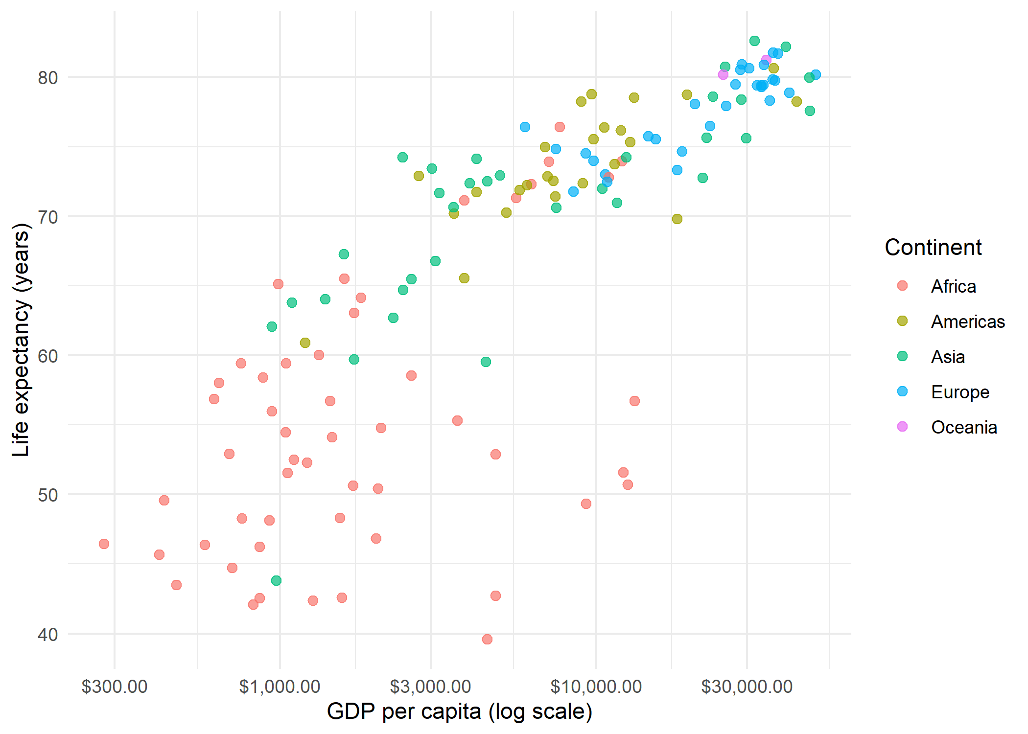

Even with log scaling, the low-GDP region (below $5,000) is densely packed and hard to read. This is exactly the situation where facet_zoom() shines.

Basic zoom

The simplest usage specifies an xlim to define the region of interest. The result is a two-panel plot: the original on one side and the zoomed view on the other.

p_base +
  facet_zoom(xlim = c(100, 5000))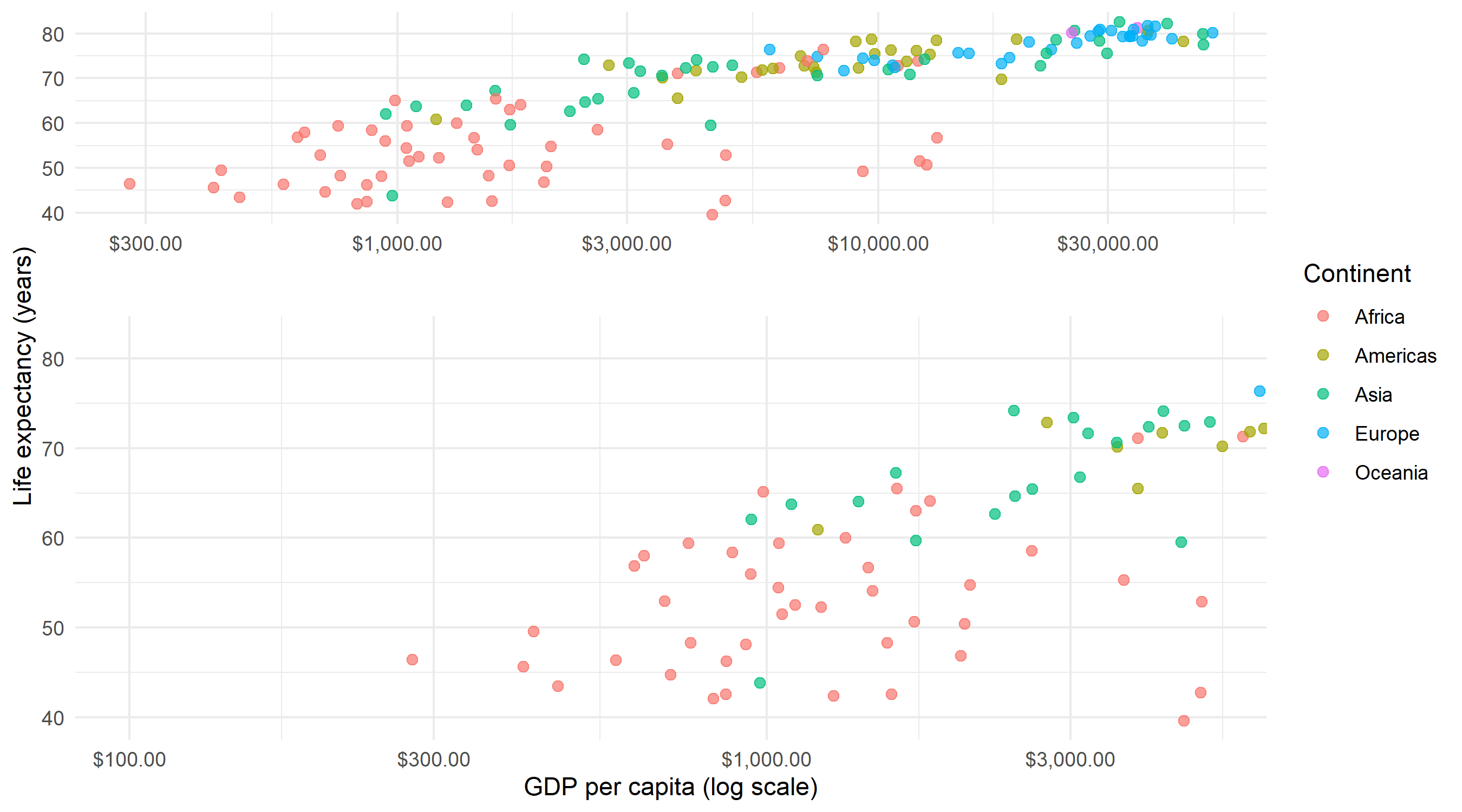

The zoom panel shows only countries with GDP per capita between $100 and $5,000, making it much easier to distinguish individual points in this crowded region. A shaded rectangle in the overview panel indicates which area is being magnified.

Styled zoom

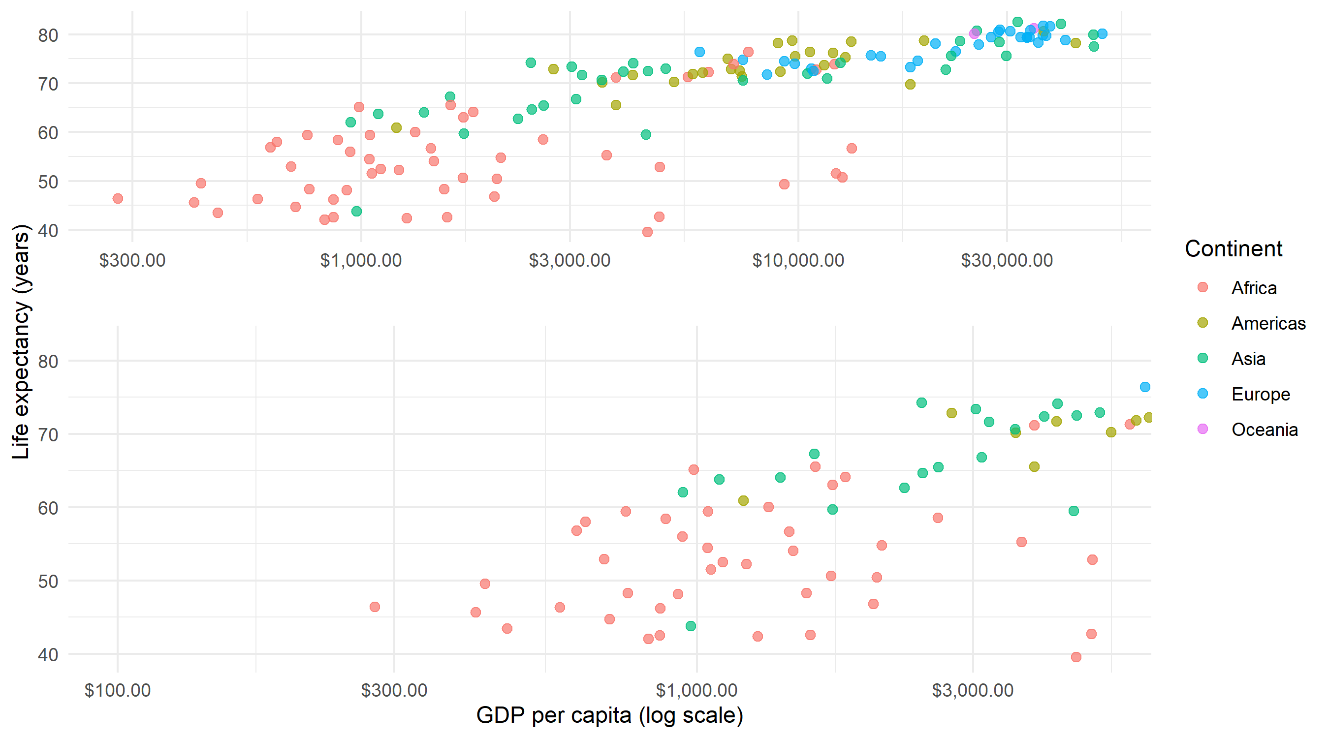
Two useful parameters control the appearance: zoom.size adjusts the relative size of the zoom panel (values greater than 1 make it larger than the overview), and show.area = TRUE highlights the zoomed region in the overview panel with a shaded rectangle.

p_base +
  facet_zoom(
    xlim = c(100, 5000),
    zoom.size = 1.5,
    show.area = TRUE
  )

Note that facet_zoom() also accepts a ylim parameter for vertical zooming, and both can be combined to zoom into a rectangular sub-region. For most use cases, zooming along a single axis is sufficient and easier to interpret.

geom_mark_ellipse

When a scatterplot contains distinct clusters, it can be helpful to visually outline each group. geom_mark_ellipse() draws a statistical ellipse (based on the covariance matrix) around the points of each group. This is particularly effective for presentations where one wants to emphasize group separation.

Basic ellipse

The iris dataset contains measurements of sepal and petal dimensions for three species. We map Species to both color and group, and add labels via the label aesthetic.

p_iris <- ggplot(iris, aes(x = Sepal.Length, y = Sepal.Width, color = Species)) +
  geom_point(size = 2, alpha = 0.7) +
  theme_minimal()

p_iris +
  geom_mark_ellipse(aes(label = Species, group = Species))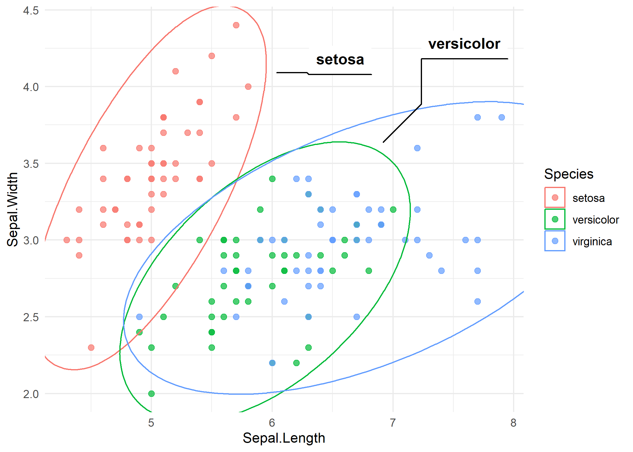

Each ellipse encloses the points of one species, and a label is placed outside the ellipse with a connector line. The ellipse shape reflects the bivariate distribution of each group - elongated ellipses indicate correlated variables within that group.

Styled ellipse

Several parameters control the appearance. expand adds padding around the ellipse, con.type changes the connector style (“elbow”, “straight”, or “none”), and the description aesthetic adds a secondary label below the main one. Here we add the number of observations per species as a description.

iris_desc <- iris %>%
  group_by(Species) %>%
  mutate(desc = glue::glue("n = {n()}")) %>%
  ungroup()

ggplot(iris_desc, aes(x = Sepal.Length, y = Sepal.Width, color = Species)) +
  geom_point(size = 2, alpha = 0.7) +
  geom_mark_ellipse(
    aes(label = Species, group = Species, description = desc),
    expand = unit(3, "mm"),
    con.type = "straight"
  ) +
  theme_minimal()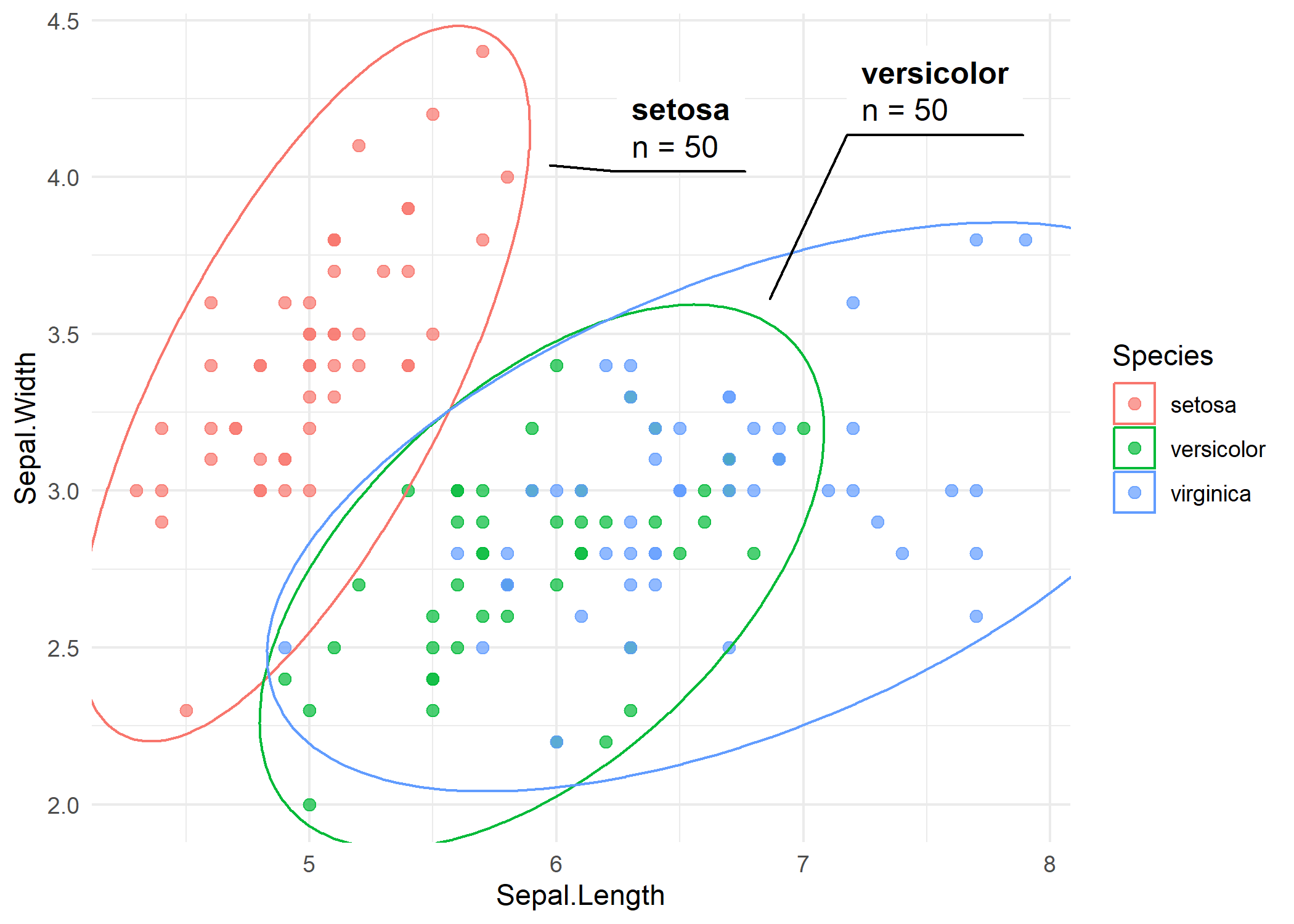

The straight connectors give a cleaner look, and the description line provides additional context without cluttering the plot.

geom_mark_hull

While ellipses assume an approximately normal distribution, convex hulls trace the actual boundary of each group’s points. This makes geom_mark_hull() a better choice when groups have irregular shapes or when one wants to highlight the precise extent of the data rather than an idealized statistical shape.

Basic hull

The syntax mirrors geom_mark_ellipse():

p_iris +
  geom_mark_hull(aes(label = Species, group = Species))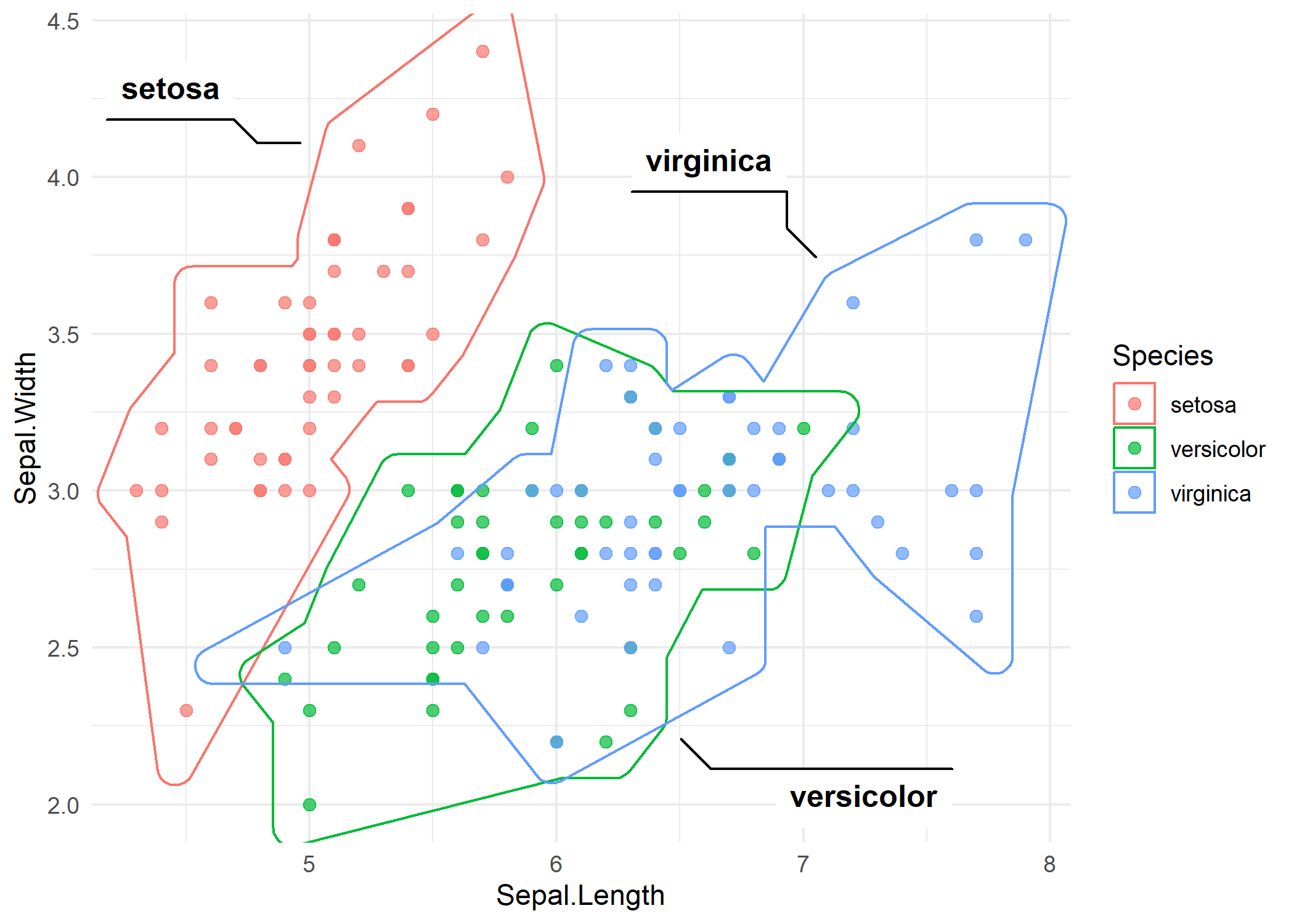

The hull wraps tightly around the outermost points of each group. Compared to the ellipses, the hull follows the actual data boundary - notice how the setosa hull is more compact because the points are tightly clustered.

Styled hull

The expand and radius parameters control padding and corner rounding, respectively. Increasing both values produces a smoother, more visually appealing shape.

p_iris +
  geom_mark_hull(
    aes(label = Species, group = Species),
    expand = unit(3, "mm"),
    radius = unit(3, "mm")
  )

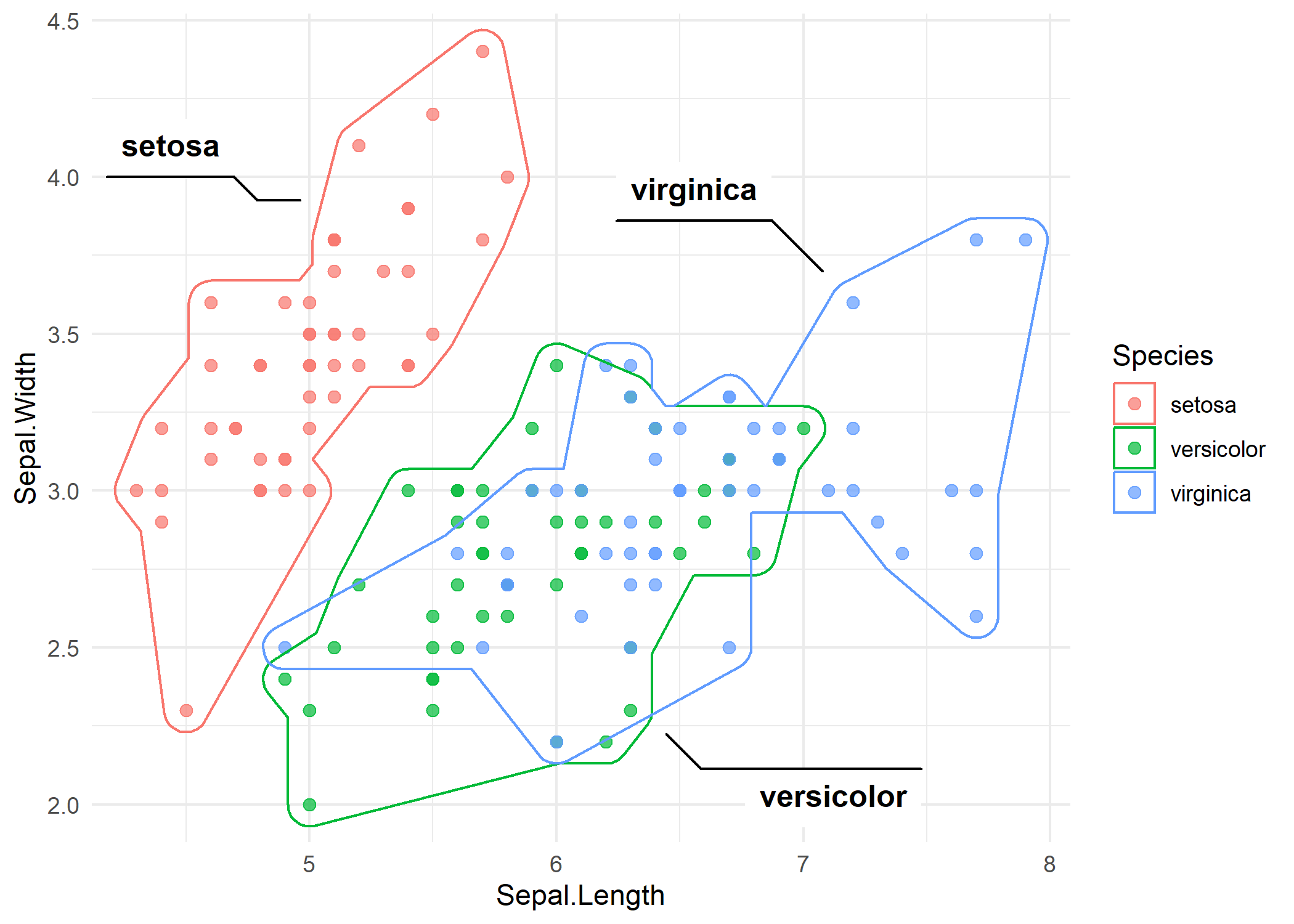
The rounded corners make the hulls look less angular and more polished, which is often preferable in presentations and publications.

TipEllipse vs. Hull vs. Rect - when to use which?

The ggforce package offers three group-marking geoms, each suited to different situations:

• geom_mark_ellipse(): Best when groups are roughly normally distributed. The ellipse reflects the statistical spread and orientation of each cluster. Useful for conveying distributional properties.
• geom_mark_hull(): Best when one wants to highlight the actual extent of the data without any distributional assumption. The hull follows the outermost points exactly (with optional smoothing).
• geom_mark_rect(): The simplest option - a rectangular bounding box around each group. Useful when groups are well-separated and a simple highlight is sufficient.

All three accept the same core aesthetics (label, group, description) and styling parameters (expand, con.type), so switching between them is straightforward.