To install and load all the packages used in this chapter, run the following code:
Introduction to R Projects
Before we dive into the specifics of importing and exporting data, it’s important to understand how R projects can make your life much easier when working with files outside of R.
Setting up R Projects
R Projects are a feature of RStudio that help you organize your work. They keep all files associated with a particular analysis together - data, R scripts, results, figures - in one directory. This has several advantages:
- Better organization of your work
- Easier collaboration with others
- Simplified path handling when importing and exporting data
To create a new R Project:
- In RStudio, go to File -> New Project
- Choose either “New Directory” or “Existing Directory” depending on your needs. (I have usually already created a new folder beforehand and then select “Existing Directory” in this step.)
- Follow the wizard to complete the setup
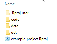
To check whether this worked as intended you can check two things: (1) In the top right corner of R-Studio you should now see the name of the folder you selected as your R-project folder. (2) Outside of R-Studio, in your file explorer, you should see a file with the extension .Rproj in the folder you selected. This file is the R-project file and it contains all the information about your project.
The main advantages of taking the extra steps to create an R-project are:
-
Automatic Working Directory: When you open an R Project, the so called working directory is automatically set to the project folder. The working directory is basically the location/folder on your computer, where R looks for files to read in and where it saves files to. Before you set up an R-project this working directory is probably in some random location on your computer - you can find out by running the code
getwd()in the console. - Project Management: R Projects help you manage your files and scripts in a structured way. You can easily switch between projects without worrying about file paths or working directories. A project even remembers which R scripts you had open when you last closed the project, so you can pick up right where you left off. Even sharing an entire project with someone else is easy, as you can just send them the entire folder and they can open it in RStudio. This is a lot easier than sending them a bunch of files and telling them to put them in the right place on their computer.
- Version Control: A more advanced thing would be to integrate with version control systems like Git, making it easier to track changes and collaborate with others. However, we will not cover this in this introductory course.
Check out the official RStudio explanation on Using RStudio Projects and Chapter 1.6 Projects in RStudio in the book “An Introduction to R”
Organizing with Subfolders
It is not strictly necessary, but a good practice to organize your R Project folder with a consistent folder structure, i.e. with subfolders like
-
data/: For raw and processed data files -
code/orR/: For your R scripts and functions -
out/orresults/: For outputs like plots, tables, and analysis results
This organization makes it easier to find your files and maintain a clean workflow.
From this moment on, the code you see will only work if you have created an R-project and that you have created the subfolders data/, out/, and code/ inside of it. Thus, the main folder name (i.e. R-project name) can be whatever you chose, but the names of the subfolders and files inside the subfolders must be identical on your PC as compared to the ones here in order for the code to work. If you want to use different names, you can do so, but then you have to change the code accordingly. Here is a screenshot of what it should look like inside your R-project folder right now:
Moreover (!), you must download the files that are available here on GitHub (Download-Link). These files should then be saved inside your data folder:
- an_excel_file.xlsx
- Clewer&Scarisbrick2001.csv
- Mead1993.csv
- vision fixed.xls
- vision.xls
- yield_increase.csv
The {here} Package
Again - not strictly necessary, but a good practice: The {here} package is a great tool for managing file paths in R projects. It automatically detects your project root directory allows you to create file paths relative to it, making your code more portable and easier to share with others. For example, assuming there was a file mydata.xlsx inside the data-subfolder, you could simply write
here("data", "mydata.xlsx")Moreover, the {here} package is very useful for creating file paths that are platform-independent. This means that you can use the same code on different operating systems (Windows, Mac, Linux) without worrying about differences in file path syntax.
CSV
One of the simplest ways to get started with data import is to read directly from a URL. This approach doesn’t require you to download files and would also work without having an R project set up. For example, you can import the following CSV-file like so:
  variety yield row col
1      v1 25.12   4   2
2      v1 17.25   1   6
3      v1 26.42   4   1
So, given your internet connection is working, you can run this code anywhere and it will work. First, we are saving the URL where the file is stored (as a string using ") into a variable x. Then, we pass that variable to the import function read.csv(). You could of course also just paste the URL directly into the function.
Note that you could also just paste that URL in your browser and see the file - it really is just a csv file but instead of being on your computer, it is on the internet.
Importing
Moreover, we see that the function that did the importing is called read.csv(). This is a function that is part of base R, which means it is built-in and does not require any additional packages. Most importing functions in R start with read. and end with the file type they are designed to read/import. CSV is short for “Comma-Separated Values” and is a common format for storing tabular data. It is a plain text file that (usually) uses commas to separate values - again, feel free to follow the URL above and actually look at the data. You will find that indeed it simply includes all the data points per line, separated by commas.
After our successful import, we can see that the data is now stored in a variable called mydf. This variable is a data frame because read.csv() is a base R function and so it imports to the base R data type for tables: data.frame. Note that the tidyverse also has its own package just for importing data called readr. This package is part of the tidyverse and is designed to be faster and more user-friendly than base R functions. In order to use its function instead, you would need to use the function read_csv() instead of read.csv(). As you may have expected, it imports to the tidyverse data type for tables: tibble. Furthermore, it also shows some additional information about the data when importing:
mytbl <- read_csv(file = x) # import dataRows: 24 Columns: 4
── Column specification ────────────────────────────────────────────────────────
Delimiter: ","
chr (1): variety
dbl (3): yield, row, col
ℹ Use `spec()` to retrieve the full column specification for this data.
ℹ Specify the column types or set `show_col_types = FALSE` to quiet this message.head(mytbl, n = 3) # view first rows of data# A tibble: 3 × 4
variety yield row col
<chr> <dbl> <dbl> <dbl>
1 v1 25.1 4 2
2 v1 17.2 1 6
3 v1 26.4 4 1Note that in our case, the only information the functions need to import this dataset is its location/path. This path can either be a URL like above or a file path on your computer. However, there are several arguments you can add to the function to customize the import process. For example, you can specify whether the first row of the file contains column names or not, what character/symbol is used to separate values, how to handle missing values or even whether the first few rows in the data should be skipped. All this can save you from having to manually fix the data before importing. You can find out more by running ?read.csv() or ?read_csv() and going through the help page.
Exporting
As you may have guessed, the function for exporting data is called write.csv(). As opposed to the import functions, it needs at least two pieces of information: The data you want to export and the location/path where you want to save it. The function will then create a CSV file at that location. So in order to export e.g. our table mytbl, we would run the following code:
As you can see, we are using the here-function we introduced earlier to create the file path. Running this creates a csv file named mytbl.csv in the data-subfolder of your R-project folder. Again, there are several additional arguments you can add to the function to customize the export process. For example, you can specify whether to include row names or not by setting the argument row.names = FALSE. By default this is set to TRUE so rownames are exported, as you can see in the data (or the screenshots of the data below).
Congratulations, you have now successfully imported and exported data in R! Most of what follows now are just different versions of this same process.
Here is a quite irritating fact about CSV files and Microsoft Excel. While we did just export a perfectly fine CSV file, notice that if you open it in Excel, it may not look fine as the columns are not separated correctly:
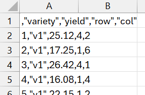
This is because Excel uses semicolons (;) instead of commas (,) as separators in many regional settings, despite CSV standing for “Comma-Separated Values”. This does make sense e.g. for Germany, where a comma is used as a decimal separator: One half is 0,5 instead of 0.5 so if you were to use a comma as a separator, it wouldn’t work properly.
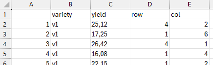
So if you are creating a CSV file that needs to be opened in Excel (in the respective regional setting), you can use the function write.csv2() instead of write.csv(). This function uses semicolons as separators and will create a CSV file that opens correctly in Excel. You can also use the read.csv2()/read_csv2() functions to import such files.
write.csv2(
  x = mytbl,
  file = here("data", "mytbl.csv")
)
TXT
Text files (.txt) are very similar to CSV files, with the main difference being that they often use a tab character (tabulator) as a delimiter rather than a comma. In essence, both are plain text formats that store tabular data - they just use different characters to separate the values.
To import a tab-delimited text file, we can use the more general read.delim() function in base R or read_delim() in the tidyverse. Note that the following codes are just examples and will not work unless you have a file named mydata.txt in the data-subfolder of your R-project folder.
# Base R approach
txt_data_base <- read.delim(file = here("data", "mydata.txt"), sep = "\t")

# Tidyverse approach
txt_data_tidy <- read_delim(file = here("data", "mydata.txt"), delim = "\t")
Exporting text files follows a similar pattern to CSV files:
# Base R approach
write.table(x = mytbl,
            file = here("data", "mytbl.txt"),
            sep = "\t")

# Tidyverse approach
write_delim(x = mytbl,
            file = here("data", "mytbl.txt"),
            delim = "\t")
The delim and sep arguments let you specify which character should separate values in your output file. Common delimiters include tabs ("\t"), commas (","), semicolons (";"), and even spaces (" ").
Since CSV and TXT files are both essentially plain text formats with different separators, the same principles apply to both. Now that we’ve covered these simple text-based formats, let’s move on to working with more complex file types like Excel.
Excel
Importing Excel Files with {readxl}
Excel files (.xlsx, .xls) are very commonly used in many fields. They support multiple worksheets, formatting, formulas, and much more. To import Excel files into R, we use the {readxl} package, which we have already loaded at the beginning of this chapter.
Please make sure you have downloaded the Excel file an_excel_file.xlsx from the course website and placed it in the data-subfolder of your R-project folder. Otherwise, the code below will not work.
xlsx_path <- here("data", "an_excel_file.xlsx")dat_sheet1 <- read_excel(path = xlsx_path)
dat_sheet1# A tibble: 3 × 2
Name Value
<chr> <dbl>
1 A 12
2 B 13
3 C 12This function attempts to read the first sheet in the Excel file by default. If your data is in another sheet, you need to specify it. We can find out all sheet names in the file with the excel_sheets() function:
excel_sheets(path = xlsx_path)[1] "data1" "otherdata"and then import the second sheet either by name or by index:
# Read a specific sheet by name
dat_sheet2 <- read_excel(path = xlsx_path, sheet = "otherdata")

# Or by sheet index
dat_sheet2 <- read_excel(path = xlsx_path, sheet = 2)

dat_sheet2
Similar to CSV imports, you can customize how the data is imported with additional arguments like col_names, na, etc. You can even select a specific range of cells to be imported via e.g. range = "A1:C10". Check the documentation with ?read_excel for more details.
Exporting to Excel with {openxlsx}
For exporting data to Excel format, we use the {openxlsx} package, which we loaded at the beginning. This package provides two main approaches: a simple one-liner function, and a more detailed approach for greater control. And yes, we are using two different packages here: readxl for importing and openxlsx for exporting excel files.
One Table to One Sheet
The easiest way to export a data frame to Excel is:
write.xlsx(x = mytbl, file = here("data", "exported_data.xlsx"))As you can see this feels very much like write.csv(), write_delim() etc., which is nice.
Multiple Tables to Multiple Sheets
For more control over the Excel file’s appearance, you can use a more detailed approach. Say we want to create an excel file with two sheets called “SheetA” and “SheetB”. The first one should contain mytbl, while the second one should contain the PlantGrowth data. The minimal code for this would look like:
# Create a new workbook
mywb <- createWorkbook()

# Sheet A
addWorksheet(wb = mywb, sheetName = "SheetA")
writeData(wb = mywb, sheet = "SheetA", x = mytbl)

# Sheet B
addWorksheet(wb = mywb, sheetName = "SheetB")
writeData(wb = mywb, sheet = "SheetB", x = PlantGrowth)

# Save the workbook
saveWorkbook(wb = mywb, here("data", "formatted_excel.xlsx"), overwrite = TRUE)
So as you can see, we are creating a so-called workbook first, then adding sheets to it and writing data to those sheets. Finally, we save the workbook to a file. The overwrite = TRUE argument allows you to overwrite an existing file with the same name.
Note that this is by far not everything you can achieve with the openxlsx package. You can also format cells, add charts, and much more. Check out the documentation for more details.
Other File Formats
While CSV and Excel are the most common file formats, you might encounter other types in your work. Here are some packages for handling those:
-
Statistical Software: The
havenpackage can import/export SPSS (.sav), SAS (.sas7bdat), and Stata (.dta) files.
Databases: Packages like
DBI,RSQLite, andRMySQLprovide connections to various database systems.JSON & XML: The
jsonliteandxml2packages handle these web-oriented formats.Specialized Formats: For field-specific formats, search CRAN for appropriate packages - there’s likely a solution for your needs.
In most cases, the functions for importing/exporting these formats follow similar patterns to what we’ve seen with CSV and Excel, starting with read_ or write_ followed by the format name.
Exporting Plots via ggsave()
I know we have not actually learned how to create a ggplot, but since we are talking about im- and exporting, we will also cover how to export plots.
While RStudio’s “Export” button in the Plots pane works, the ggsave() function provides a more reproducible approach.
Let’s first create a simple plot for demonstration, once again using the PlantGrowth dataset:
# Create a sample plot
myplot <- ggplot(data = PlantGrowth, aes(x = group, y = weight)) +
  geom_boxplot()

# Display the plot
myplot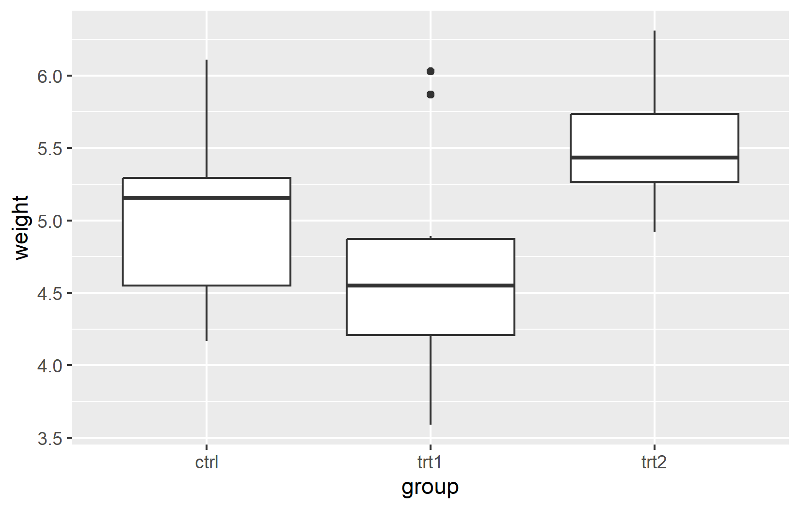
Now we can export this plot using ggsave():
The ggsave() function has several important arguments:
- filename: The name of the file (including extension)
- plot: The plot object to save (defaults to the last displayed plot if not specified)
- path: Where to save the file
- width, height: Dimensions of the image
- units: Unit for width/height (“cm”, “in”, “mm”, etc.)
- dpi: Resolution in dots per inch (higher = better quality but larger file)
The file extension in the filename determines the output format. Above, we exported a PNG, but we may just as well export a PDF or SVG, which are vector formats. Vector formats are ideal for publication-quality figures, as they can be resized without losing quality. The only thing you need to change is the file extension in the filename argument.
When choosing a file format for your plots:
- PNG (.png): Good for presentations and web use
- JPEG (.jpg): Smaller file size but lower quality
- PDF (.pdf): Vector format ideal for publications and printing
- SVG (.svg): Vector format good for web use and further editing
- TIFF (.tiff): High-quality format often required by journals
For publication-quality figures, PDF or TIFF are usually preferred. For presentations or web use, PNG often works best.
Faster Alternatives for Large Data
While the functions we’ve covered so far are perfectly adequate for most everyday data analysis tasks, when working with very large datasets (with millions of rows), you may notice that importing takes noticeably longer. For such cases, there are specialized packages designed to read data much faster.
The {data.table} Package
The {data.table} package is well-known for its extremely fast fread() function (short for “fast read”). This function can often import CSV files 5-10 times faster than the standard functions:
# Install and load data.table if needed
# install.packages("data.table")
library(data.table)

# Very fast import of CSV files
fast_data <- fread(file = "some_large_dataset.csv")
In addition to fast importing, fread() creates a data.table object that is also optimized for very fast data manipulation. However, if you need the data as a regular data.frame or tibble, you can easily convert it.
The {vroom} Package
The {vroom} package is another alternative that’s part of the extended tidyverse ecosystem. It specializes particularly in reading very large files extremely quickly:
What’s special about vroom() is that it uses a so-called “lazy loading” approach - it doesn’t immediately read all data into memory, but only the parts you actually use. This can be advantageous when working with gigantic datasets.
For normal data analysis projects with datasets that have fewer than 100,000 rows, the standard import functions are completely sufficient. The specialized speed packages only become truly useful with very large data (millions of rows) or when repeatedly importing the same large file.
If you’re interested in these powerful alternatives, you should check out the respective package documentation, as they also offer advanced features for data manipulation that go beyond simple importing.
Wrapping Up
You now know how to efficiently move data in and out of R, a fundamental skill that will save you countless hours in your data analysis journey.
R Projects provide a robust framework for organizing your work, managing file paths, and ensuring reproducibility.
-
For data import/export:
- CSV files: Use
read.csv()/write.csv()(base R) orread_csv()/write_csv()(tidyverse) - TXT files: Use
read.delim()/write.table()(base R) orread_delim()/write_delim()(tidyverse) - Excel files: Use
read_excel()from {readxl} for import andwrite.xlsx()from {openxlsx} for export
- CSV files: Use
The {here} package simplifies file path management, making your code more portable and easier to share.
-
When working with Excel files, be aware that you can:
- Read specific sheets by name or index
- Export multiple tables to different sheets within the same workbook
For plots, use
ggsave()to export in various formats (PNG, PDF, SVG) with precise control over dimensions and quality.Always organize your project with a consistent folder structure (data/, code/, out/) to maintain a clean workflow.
Citation
@online{schmidt2026,
  author = {{Dr. Paul Schmidt}},
  publisher = {BioMath GmbH},
  title = {3. {Importing} \& {Exporting} {Data}},
  date = {2026-06-08},
  url = {https://biomathcontent.netlify.app/content/r_intro/03_importexport.html},
  langid = {en}
}