2+3[1] 5This chapter is mostly aimed at people who are very new to R. However, people who do know R may still find useful insights from the sections where I emphasize how I personally use R. Before you continue, make sure you have R and RStudio installed and you have watched this chapter’s video on the basics of RStudio - more specifically you should know how to use the most important panels like the Console, the Script editor and the Environment.
This is probably not the best tutorial you’ll ever find, so if you want other tutorials check out this curated list of R Tutorials here.
This document shows R code in grey boxes and the resulting output in green boxes below. Thus, you should always be able to obtain the same result you see in a green box, given you ran the same code in (all previous) grey boxes.
You can use R like a calculator. If you write and execute simple operations like so, it will return the result in the console:
2+3[1] 5As you can see, the result (i.e. 5) appears after [1] in this case. We will get back to why that is in a bit but for now you can just ignore the [1].
In R, it usually does not matter if and how many spaces you put between your numbers, operators etc. Thus, the following code would also work:
2 + 3[1] 5Accordingly, it is up to your personal preference e.g. whether you want to have spaces before and after operators like +, - etc. or not.
You can add comments to your code by using the # symbol. In any given line, everything after the # symbol will be ignored by R. This is useful as you can write notes to yourself or others at the exact position where they are relevant. For example:
2 + 3 # this is adding 2 + 3[1] 5Similar to what you may know from Microsoft Excel, you can use functions in R. The first example shall be sqrt() to obtain the square root of a number:
sqrt(9)[1] 3Again - just like in MS Excel - a function works by writing its name, then parentheses () and (usually) at least one piece of information inside the parentheses. If you are wondering how a specific function works, you can always (even without internet connection) have a look at the documentation, i.e. the manual provided by the authors of the respective functions by executing the function name with a question mark in front of it like so:
?sqrtNote that if that does not work, you may try having two questions marks in front of it, i.e. ??sqrt. This is necessary if you are looking for a function whose package you have not loaded yet. We will talk later about what a package is.
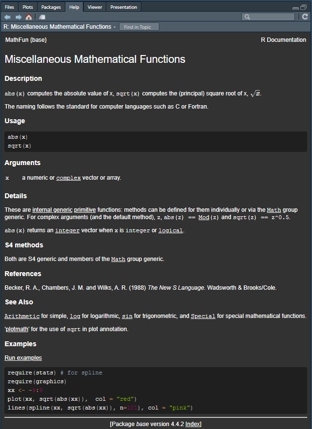
The documentation will show up in the Help panel in RStudio (see screenshot below) and contain quite a bit of information about this function. In fact, it may be overwhelming, but it should be realized that the structure of each function’s documentation is always the same, i.e. first comes a description, then the Usage and Arguments etc. and usually some example code at the end.
Besides built-in functions, R also knows certain things like \(\pi\) or the alphabet, which are stored in the built-in constants named pi and letters. Note that these do not have parentheses
pi[1] 3.141593letters [1] "a" "b" "c" "d" "e" "f" "g" "h" "i" "j" "k" "l" "m" "n" "o" "p" "q" "r" "s"
[20] "t" "u" "v" "w" "x" "y" "z"If you want to execute code written in your script, you can either or click on the Run button in the top right corner of the script editor or press Ctrl + Enter. Moreover, if you did not highlight a specific part of your code, doing so will run the code in the line where your cursor is at and afterwards jump the cursor to the next line. However, if you did highlight a specific part of your code before executing, only that part will be executed.
While having those constants is useful, it is much more relevant to define your own variables in R. This is done by using either the assignment operator <- or the equals sign =1. The former is more common in R, but the latter is also used in other programming languages like Python.
Here is an example. Running the following code will not return anything in the console, but it will store the number 5 in the variable x:
x <- 5To check whether the variable x has been created and what it contains, you can simply type x in the console and press Enter:
x[1] 5As said before, we may also use the equals sign = to assign a value to a variable:
y = 10
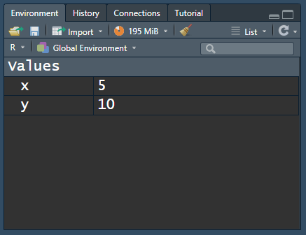
y[1] 10Note also that you can see all defined variables by looking at the Environment panel in RStudio. This panel shows all variables and their values that you have defined so far.
Note that a variable can be overwritten by assigning a new value to it. For example, if we now assign the value 7 to x, the value of x will be overwritten:
x # show the current value of x[1] 5x <- 7 # overwrite the value of x
x # show the new value of x[1] 7You can also perform operations with variables. For example, if you have defined x and y as above, you can add them together:
x + y[1] 17Furthermore, you can also assign the result of an operation to a new variable. For example, if you want to add x and y and store the result in a new variable z, you can do so like this:
z <- x + y
z
[1] 17Note also that variables can hold all kinds of information, not just numbers as in the examples above. Moreover, in practice, you may want to use more descriptive variable names than x, y and z. For example, you could use a variable name like mytext to store a text:
mytext <- "This is my text"
mytext
[1] "This is my text"As you can see, the difference between writing text to function as a variable name and as a piece of text is that the text is written in quotation marks. This is how R knows that you are not referring to a variable but to a piece of text. You may either use " or ' for this purpose, but it is important to use the same type of quotation mark at the beginning and the end of the text. Note that those pieces of text are called strings in programming.
As you just saw, R can deal with both numbers and text and actually many more types of data. Each variable does not only hold the value you assigned to it, but also information about the type of data it holds. We can check the data type of a variable via the typeof() function:
As you can see, x is of type double and mytext is of type character. Here is a simplified overview over some of R’s data types you may see more often:
Here is a simplified overview over some of R’s data types you may see more often:
integer/int: whole numbernumeric/num & double/dbl: real numbercharacter/chr: string valuesfactor/fct: categorical variable that stores both string and integer data values as “levels”logical/logi: logical valueInstead of working with individual numbers or pieces of text, we obviously need to work with entire datasets. Before we get to a full table with multiple rows and columns, the first step is to understand what a vector is in R: It is a sequence of elements that share the same data type. You can also think of it as a single column in a dataset. Above, we actually already looked at a vector: letters is a vector with 26 elements of data type character. We could verify this using the length() or str() functions:
length(letters)[1] 26str(letters) chr [1:26] "a" "b" "c" "d" "e" "f" "g" "h" "i" "j" "k" "l" "m" "n" "o" "p" ...This is also a good opportunity to get back to the [1] we have ignored so far. When printing the letters vector to the console, you probably see more than just [1]:
letters [1] "a" "b" "c" "d" "e" "f" "g" "h" "i" "j" "k" "l" "m" "n" "o" "p" "q" "r" "s"
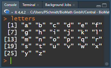
[20] "t" "u" "v" "w" "x" "y" "z"In fact, you see one of these numbers in square brackets at the beginning of each line. This is the index of the element in the vector. The first element has index 1, the second element has index 2, and so on. So here we see a [1] because "a" is the first element of this vector, and a [20] because "t" is the twentieth element of this vector. Note that it depends very much on the width of your console as well as the font size etc. how many elements you see in one line. Here is a screenshot of what it looks like in RStudio when I make my console very narrow and then print letters again:
Accordingly, these numbers in brackets in the console output are really just for orientation. However, we can actually access a single element of a vector by using exactly these numbers in square brackets. For example, if you want to access the third element of the letters vector, you can do so like this:
letters[3][1] "c"If you want to create a vector yourself, you write all elements into the c() function and separate them with commas:
mynumbers <- c(1, 4, 9, 12, 12, 12, 16)
mynumbers
[1] 1 4 9 12 12 12 16mywords <- c("Hakuna", "Matata", "Simba")
mywords[1] "Hakuna" "Matata" "Simba" Interestingly, we can also apply the sqrt() function we used above to a vector of numbers, and it will simply take the square root of each element:
sqrt(mynumbers)[1] 1.000000 2.000000 3.000000 3.464102 3.464102 3.464102 4.000000However, there are also functions like mean() that return the average of all numbers in a vector as a single output element:
mean(mynumbers)[1] 9.428571In R, comparison operators are used to compare values and variables, much like you might in mathematics or in spreadsheet formulas. They are fundamental in making decisions and controlling the flow of your code. Here are the most commonly used comparison operators:
==): Checks if the values on either side are equal.!=): Determines if two values are different.<): Verifies if the value on the left is smaller than the one on the right.>): Checks if the value on the left is larger than the one on the right.<=): True if the left value is less than or equal to the right value.>=): True if the left value is greater than or equal to the right value.Here are some examples:
5 == 5[1] TRUE3 < 4[1] TRUE5 <= 5[1] TRUE5 != 5[1] FALSE2 > 6[1] FALSE5 >= 4[1] TRUESo far, the functions we used had in common that they required only one input. The really good stuff in R happens with more complex functions which need multiple inputs. Let us use seq() as an example, which seems simple enough, because it generates a sequence of numbers:
seq(1, 10) [1] 1 2 3 4 5 6 7 8 9 10As you can see, putting in 1 and 10 separated by a comma generates a numeric vector with numbers from 1 to 10. However, I would like you to fully understand what is going on here, because it will help a lot with more complex functions.
See, we could switch the numbers and the function will work as expected:
seq(10, 1) [1] 10 9 8 7 6 5 4 3 2 1So this means that the first input is always the starting point and the second one is always the end point of the sequence, right? Well, yes by default, but you can have it your way if you specifically use the names of the arguments. The individual inputs of a function are called arguments and you can always look up the order of the arguments and their names in the documentation of a function.
Looking at ?seq() it says seq(from = 1, to = 1, by = ...) so this seq(1, 10) is more explicitly this: seq(from = 1, to = 10, by = 1). Here is proof that you could also write the function with explicit argument names and it will return the exact same result:
seq(from = 1, to = 10, by = 1) [1] 1 2 3 4 5 6 7 8 9 10Again: if you do not write out the arguments like this, it will simply assume the default order: The first number supplied is from = the second is to = and the third is by = - that’s just how this function was created/programmed. However, if we write out the argument names, we can rearrange them and use any order we like:
seq(1, 9, 2) # Example A[1] 1 3 5 7 9seq(from = 1, to = 9, by = 2) # Example B[1] 1 3 5 7 9seq(from = 1, by = 2, to = 9) # Example C[1] 1 3 5 7 9seq(1, 2, 9) # Example D[1] 1In short: If you understand why the Examples A-C above produce the same result, but Example D does not, you are good to go!
Any function you will ever use in R is always part of an R package. An R package is a collection of functions, data, and documentation.
The functions we have used so far are part of the so-called base R. This is the set of functions/packages that comes with every installation of R. Even if you just installed R, you will quite a number of packages already available to you by looking at the Packages panel in RStudio. Here you can see all the packages you have installed and you can also see which ones are loaded. A loaded package is shown with a checkmark in front of it. If you want to use a function from a package, you must load the package first. However, as said before, you do not need to load the base R functions/packages, because they are always loaded, which is why we were able to use the functions above.
To load a package, you can use the library() function. For example, there is a package called tools which is installed on your computer by default, but not loaded. If you want to use a function from this package, you must load it first.
library(package_name_here)This command must be run once every time (!) you open a new R session, which basically means every time you open RStudio.
R really shines because of the ability to install additional packages from external sources. Basically, anyone can create a function, put it in a package and make it available online. Some packages are very sophisticated and popular - e.g. the package ggplot2, which is not built-in, has been downloaded 168 million times. In order to install a package, the default command is install.packages("package_name"). Alternatively, you can also click on the “Install” button in the top left of the Packages tab and type in the package_name there.
install.packages("package_name_here")Once you have successfully installed a package, it will show up in your list of packages in the Packages tab. However, it will not have a check mark, which means you must still load it with the library() function if you want to use its functions:
Check out Chapter Chapter 1 Getting started with R and RStudio in the book “An Introduction to R”
Congratulations! You’ve completed your introduction to R fundamentals and have taken your first steps into the world of R programming. You now have the basic skills needed to start writing and executing your own R code.
R can be used as a calculator with operations like addition (+), subtraction (-), multiplication (*), and division (/).
Variables allow you to store values for later use:
<-) or equals sign (=) to create variablesFunctions are essential tools in R:
?function_name
R has several important data structures:
vector[3])c() functionComparison operators like ==, !=, <, > return logical values (TRUE/FALSE)
R packages extend functionality:
install.packages("package_name")
library(package_name)
Use comments with # to document your code and make it more understandable
Does it make a difference whether I use <- or =? The short answer is no. The more precise answer is in this video.↩︎
@online{schmidt2026,
  author = {{Dr. Paul Schmidt}},
  publisher = {BioMath GmbH},
  title = {1. {R/RStudio} {Fundamentals}},
  date = {2026-06-08},
  url = {https://biomathcontent.netlify.app/content/r_intro/01_fundamentals.html},
  langid = {en}
}