To install and load all packages used in this chapter, run the following code:

for (pkg in c("tidyverse")) {
  if (!require(pkg, character.only = TRUE)) install.packages(pkg)
}

library(tidyverse)

Introduction

In practice, data rarely comes in a single, perfectly prepared table. Instead, we often have multiple data sources that need to be combined: measurements from different laboratories, master data and transaction data, or simply data spread across multiple Excel sheets. This chapter shows how to combine tables in R using various approaches.

We distinguish three fundamental approaches:

Stacking: Simply placing tables below each other (bind_rows()) or next to each other (bind_cols())
Joining: Intelligently linking tables based on common key columns
Reshaping: Transforming data between “wide” and “long” formats

Stacking Tables

The simplest way to combine tables is “stacking” - placing tables either below or next to each other. For this purpose, we have bind_rows() and bind_cols().

Example Data

For this section, we create three small tibbles with fruit data:

fruit_1 <- tibble(
  variety = c("Apple", "Pear"),
  price = c(1.20, 1.50)
)

fruit_2 <- tibble(
  variety = c("Orange", "Banana"),
  price = c(0.80, 1.10)
)

fruit_3 <- tibble(
  variety = c("Cherry", "Plum"),
  price = c(3.50, 2.20),
  origin = c("Germany", "Spain")
)

fruit_1

# A tibble: 2 × 2
  variety price
  <chr>   <dbl>
1 Apple     1.2
2 Pear      1.5

fruit_2

# A tibble: 2 × 2
  variety price
  <chr>   <dbl>
1 Orange    0.8
2 Banana    1.1

fruit_3

# A tibble: 2 × 3
  variety price origin 
  <chr>   <dbl> <chr>  
1 Cherry    3.5 Germany
2 Plum      2.2 Spain

Note that fruit_1 and fruit_2 have the same columns (variety and price), while fruit_3 has an additional column origin.

bind_rows()

The function bind_rows() stacks tables vertically - it adds rows. This is useful when you have data from different time periods or different sources that share the same structure.

bind_rows(fruit_1, fruit_2)

# A tibble: 4 × 2
  variety price
  <chr>   <dbl>
1 Apple     1.2
2 Pear      1.5
3 Orange    0.8
4 Banana    1.1

This works as expected: the rows are simply stacked on top of each other.

Different Columns

The big advantage of bind_rows() over the base R function rbind() becomes apparent when the tables have different columns. While rbind() throws an error in this case, bind_rows() combines the tables anyway and fills missing values with NA:

bind_rows(fruit_1, fruit_3)

# A tibble: 4 × 3
  variety price origin 
  <chr>   <dbl> <chr>  
1 Apple     1.2 <NA>   
2 Pear      1.5 <NA>   
3 Cherry    3.5 Germany
4 Plum      2.2 Spain

As we can see, fruit_1 had no origin column, so these values are filled with NA. This is very convenient when combining data from different sources that don’t have exactly the same columns.

Tracking Origin with .id

When combining multiple tables, we often want to know which original table each row came from. For this, there’s the .id argument:

bind_rows(
  "Store_A" = fruit_1,
  "Store_B" = fruit_2,
  .id = "source"
)

# A tibble: 4 × 3
  source  variety price
  <chr>   <chr>   <dbl>
1 Store_A Apple     1.2
2 Store_A Pear      1.5
3 Store_B Orange    0.8
4 Store_B Banana    1.1

Here we gave names to the tables (“Store_A”, “Store_B”) and created a new column with .id = "source" that contains these names.

Combining All Three Tables

We can also stack more than two tables at once:

bind_rows(fruit_1, fruit_2, fruit_3)

# A tibble: 6 × 3
  variety price origin 
  <chr>   <dbl> <chr>  
1 Apple     1.2 <NA>   
2 Pear      1.5 <NA>   
3 Orange    0.8 <NA>   
4 Banana    1.1 <NA>   
5 Cherry    3.5 Germany
6 Plum      2.2 Spain

The origin column only exists for the last two rows (from fruit_3), all others get NA.

bind_cols()

The function bind_cols() combines tables horizontally - it glues columns together.

Caution

With bind_cols() there is no intelligent linking via key columns! The tables are simply “blindly” glued together side by side. This means: the rows must be in exactly the same order, and the tables must have the same number of rows.

An example:

names_df <- tibble(
  first_name = c("Anna", "Ben", "Clara"),
  last_name = c("Mueller", "Schmidt", "Weber")
)

age_df <- tibble(
  age = c(28, 34, 22),
  profession = c("Physician", "Engineer", "Student")
)

bind_cols(names_df, age_df)

# A tibble: 3 × 4
  first_name last_name   age profession
  <chr>      <chr>     <dbl> <chr>     
1 Anna       Mueller      28 Physician 
2 Ben        Schmidt      34 Engineer  
3 Clara      Weber        22 Student

This works because both tibbles have three rows and we know that row 1 in both tibbles belongs to the same person.

When is bind_cols() Dangerous?

bind_cols() can lead to incorrect results if the row order doesn’t match:

# WRONG: Different order!
names_sorted <- names_df %>% arrange(first_name)
age_original <- age_df

bind_cols(names_sorted, age_original)

# A tibble: 3 × 4
  first_name last_name   age profession
  <chr>      <chr>     <dbl> <chr>     
1 Anna       Mueller      28 Physician 
2 Ben        Schmidt      34 Engineer  
3 Clara      Weber        22 Student

Here the names were sorted alphabetically, but the age data was not - Anna now gets age 28 assigned, which happened to be correct before sorting (and is coincidentally still correct), but Ben and Clara are swapped! This is a common mistake!

When Should You Use bind_cols()?

bind_cols() is safe when:

The data comes from the same source and is guaranteed to have the same order
You just performed multiple calculations on the same data yourself
You verify correctness after combining

In most other cases, a join is the better choice because it links via a key column.

Joining Tables

Joins are the most powerful method for combining tables. They link tables intelligently via one or more common columns (the “keys”). This means it doesn’t matter what order the rows are in - R automatically finds the matching rows.

Example Data

For the joins, we use a different dataset: city data. We create three tibbles with different information about cities:

# Tibble 1: Six major cities in Central Europe with population
cities_europe <- tibble(
  city = c("Berlin", "Hamburg", "Munich", "Copenhagen", "Amsterdam", "London"),
  population_mio = c(3.9, 1.9, 1.5, 0.7, 0.9, 9.0)
)

# Tibble 2: Ten German cities with rental prices (Euro per square meter)
cities_rent <- tibble(
  city = c("Berlin", "Hamburg", "Munich", "Frankfurt", "Cologne",
           "Duesseldorf", "Stuttgart", "Leipzig", "Dresden", "Nuremberg"),
  rent_sqm = c(18.29, 17.18, 22.64, 19.62, 15.21,
               16.04, 17.26, 11.38, 7.33, 9.65)
)

# Tibble 3: The same ten German cities with additional statistics
cities_stats <- tibble(
  city = c("Berlin", "Hamburg", "Munich", "Frankfurt", "Cologne",
           "Duesseldorf", "Stuttgart", "Leipzig", "Dresden", "Nuremberg"),
  area_km2 = c(892, 755, 310, 248, 405, 217, 207, 297, 328, 186),
  green_space_pct = c(14.4, 16.8, 11.9, 21.5, 17.2, 18.9, 24.0, 14.8, 12.3, 19.1)
)

cities_europe

# A tibble: 6 × 2
  city       population_mio
  <chr>               <dbl>
1 Berlin                3.9
2 Hamburg               1.9
3 Munich                1.5
4 Copenhagen            0.7
5 Amsterdam             0.9
6 London                9

cities_rent

# A tibble: 10 × 2
   city        rent_sqm
   <chr>          <dbl>
 1 Berlin         18.3 
 2 Hamburg        17.2 
 3 Munich         22.6 
 4 Frankfurt      19.6 
 5 Cologne        15.2 
 6 Duesseldorf    16.0 
 7 Stuttgart      17.3 
 8 Leipzig        11.4 
 9 Dresden         7.33
10 Nuremberg       9.65

cities_stats

# A tibble: 10 × 3
   city        area_km2 green_space_pct
   <chr>          <dbl>           <dbl>
 1 Berlin           892            14.4
 2 Hamburg          755            16.8
 3 Munich           310            11.9
 4 Frankfurt        248            21.5
 5 Cologne          405            17.2
 6 Duesseldorf      217            18.9
 7 Stuttgart        207            24  
 8 Leipzig          297            14.8
 9 Dresden          328            12.3
10 Nuremberg        186            19.1

Note that cities_europe contains three German cities (Berlin, Hamburg, Munich) that also appear in the other two tibbles, plus three non-German cities. The tibbles cities_rent and cities_stats have exactly the same ten German cities but different columns.

The Concept: Key Columns

In a join, you specify which column(s) should be used as “keys”. R then searches for matching values in this column and combines the corresponding rows.

In our example data, city is the obvious key column - it appears in all three tibbles and uniquely identifies each row.

Mutating Joins

“Mutating joins” add columns from one table to another - they “mutate” the source table by extending it with new columns. There are four variants that differ in which rows are included in the result.

left_join()

The left_join() keeps all rows from the left table and adds matching columns from the right table. If there is no matching partner in the right table, the new columns are filled with NA.

Source of Visualizations

The animated graphics in this chapter come from Garrick Aden-Buie. He has created a fantastic collection of visualizations there that illustrate the different join types and other tidyverse operations. Worth a visit!

cities_europe %>%
  left_join(cities_rent, by = "city")

# A tibble: 6 × 3
  city       population_mio rent_sqm
  <chr>               <dbl>    <dbl>
1 Berlin                3.9     18.3
2 Hamburg               1.9     17.2
3 Munich                1.5     22.6
4 Copenhagen            0.7     NA  
5 Amsterdam             0.9     NA  
6 London                9       NA

We can see:

All 6 cities from cities_europe are in the result
Berlin, Hamburg, and Munich have received rental prices
Copenhagen, Amsterdam, and London have NA for rent_sqm because they don’t appear in cities_rent

The left_join() is the most commonly used join because you often have a “main table” that you want to extend with additional information without losing rows.

right_join()

The right_join() is the mirror image of left_join(): it keeps all rows from the right table.

cities_europe %>%
  right_join(cities_rent, by = "city")

# A tibble: 10 × 3
   city        population_mio rent_sqm
   <chr>                <dbl>    <dbl>
 1 Berlin                 3.9    18.3 
 2 Hamburg                1.9    17.2 
 3 Munich                 1.5    22.6 
 4 Frankfurt             NA      19.6 
 5 Cologne               NA      15.2 
 6 Duesseldorf           NA      16.0 
 7 Stuttgart             NA      17.3 
 8 Leipzig               NA      11.4 
 9 Dresden               NA       7.33
10 Nuremberg             NA       9.65

Now we have:

All 10 German cities from cities_rent
Berlin, Hamburg, and Munich have population figures
The 7 other German cities have NA for population_mio

Tip

In practice, instead of right_join(a, b) you can simply write left_join(b, a) - the result is the same (only the column order differs). Many R users therefore use almost exclusively left_join().

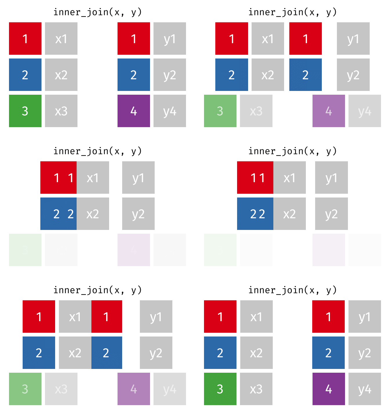
inner_join()

The inner_join() keeps only rows that appear in both tables. Rows without a partner are completely excluded.

cities_europe %>%
  inner_join(cities_rent, by = "city")

# A tibble: 3 × 3
  city    population_mio rent_sqm
  <chr>            <dbl>    <dbl>
1 Berlin             3.9     18.3
2 Hamburg            1.9     17.2
3 Munich             1.5     22.6

Only Berlin, Hamburg, and Munich remain - the only cities that appear in both tables. There are no NA values in the result.

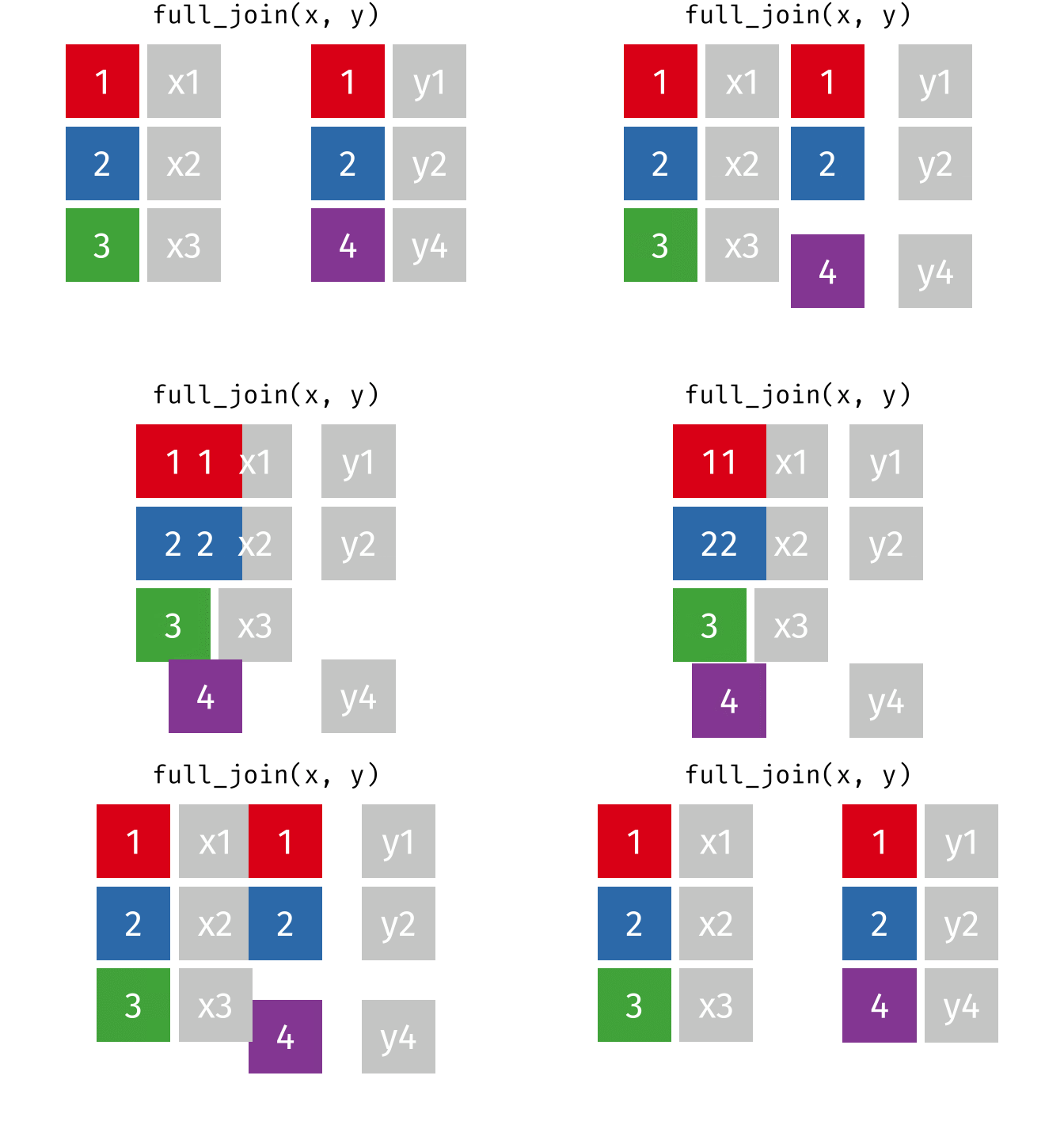
full_join()

The full_join() keeps all rows from both tables. This is the most “generous” variant.

cities_europe %>%
  full_join(cities_rent, by = "city")

# A tibble: 13 × 3
   city        population_mio rent_sqm
   <chr>                <dbl>    <dbl>
 1 Berlin                 3.9    18.3 
 2 Hamburg                1.9    17.2 
 3 Munich                 1.5    22.6 
 4 Copenhagen             0.7    NA   
 5 Amsterdam              0.9    NA   
 6 London                 9      NA   
 7 Frankfurt             NA      19.6 
 8 Cologne               NA      15.2 
 9 Duesseldorf           NA      16.0 
10 Stuttgart             NA      17.3 
11 Leipzig               NA      11.4 
12 Dresden               NA       7.33
13 Nuremberg             NA       9.65

The result has 13 rows: 3 German cities with complete data, 3 non-German cities (population only), and 7 additional German cities (rent only).

Exercise: Joins with Plant Data

First prepare the data:

# Load and extend PlantGrowth dataset
data(PlantGrowth)

# Dataset 1: Weight measurements with unique ID
plants_weight <- PlantGrowth %>%
  mutate(plant_id = 1:n()) %>%
  select(plant_id, group, weight)

# Dataset 2: Height measurements (only available for some plants!)
set.seed(123)
plants_height <- tibble(
  plant_id = c(1, 3, 5, 7, 9, 11, 13, 15, 17, 19, 21, 23, 25, 27, 29),
  height_cm = round(rnorm(15, mean = 26, sd = 3), 1)
)

# View the datasets
plants_weight

   plant_id group weight
1         1  ctrl   4.17
2         2  ctrl   5.58
3         3  ctrl   5.18
4         4  ctrl   6.11
5         5  ctrl   4.50
6         6  ctrl   4.61
7         7  ctrl   5.17
8         8  ctrl   4.53
9         9  ctrl   5.33
10       10  ctrl   5.14
11       11  trt1   4.81
12       12  trt1   4.17
13       13  trt1   4.41
14       14  trt1   3.59
15       15  trt1   5.87
16       16  trt1   3.83
17       17  trt1   6.03
18       18  trt1   4.89
19       19  trt1   4.32
20       20  trt1   4.69
21       21  trt2   6.31
22       22  trt2   5.12
23       23  trt2   5.54
24       24  trt2   5.50
25       25  trt2   5.37
26       26  trt2   5.29
27       27  trt2   4.92
28       28  trt2   6.15
29       29  trt2   5.80
30       30  trt2   5.26

plants_height

# A tibble: 15 × 2
   plant_id height_cm
      <dbl>     <dbl>
 1        1      24.3
 2        3      25.3
 3        5      30.7
 4        7      26.2
 5        9      26.4
 6       11      31.1
 7       13      27.4
 8       15      22.2
 9       17      23.9
10       19      24.7
11       21      29.7
12       23      27.1
13       25      27.2
14       27      26.3
15       29      24.3

Exercise

Answer the following questions using the appropriate join functions:

Add the height measurements to all plants. Plants without height measurement should get NA. How many plants have a height measurement?
Create a dataset with only the plants for which both weight and height were measured.
Which plants (plant_id) have no height measurement? Use a filtering join.
For the plants with both measurements, calculate the ratio weight / height_cm and store it in a new column ratio.

Solution

# a) left_join: Keep all plants, add height where available
plants_complete <- plants_weight %>%
  left_join(plants_height, by = "plant_id")

plants_complete

   plant_id group weight height_cm
1         1  ctrl   4.17      24.3
2         2  ctrl   5.58        NA
3         3  ctrl   5.18      25.3
4         4  ctrl   6.11        NA
5         5  ctrl   4.50      30.7
6         6  ctrl   4.61        NA
7         7  ctrl   5.17      26.2
8         8  ctrl   4.53        NA
9         9  ctrl   5.33      26.4
10       10  ctrl   5.14        NA
11       11  trt1   4.81      31.1
12       12  trt1   4.17        NA
13       13  trt1   4.41      27.4
14       14  trt1   3.59        NA
15       15  trt1   5.87      22.2
16       16  trt1   3.83        NA
17       17  trt1   6.03      23.9
18       18  trt1   4.89        NA
19       19  trt1   4.32      24.7
20       20  trt1   4.69        NA
21       21  trt2   6.31      29.7
22       22  trt2   5.12        NA
23       23  trt2   5.54      27.1
24       24  trt2   5.50        NA
25       25  trt2   5.37      27.2
26       26  trt2   5.29        NA
27       27  trt2   4.92      26.3
28       28  trt2   6.15        NA
29       29  trt2   5.80      24.3
30       30  trt2   5.26        NA

# Number of plants with height measurement
plants_complete %>%
  filter(!is.na(height_cm)) %>%
  nrow()

[1] 15

# b) inner_join: Only plants with both measurements
plants_both <- plants_weight %>%
  inner_join(plants_height, by = "plant_id")

plants_both

   plant_id group weight height_cm
1         1  ctrl   4.17      24.3
2         3  ctrl   5.18      25.3
3         5  ctrl   4.50      30.7
4         7  ctrl   5.17      26.2
5         9  ctrl   5.33      26.4
6        11  trt1   4.81      31.1
7        13  trt1   4.41      27.4
8        15  trt1   5.87      22.2
9        17  trt1   6.03      23.9
10       19  trt1   4.32      24.7
11       21  trt2   6.31      29.7
12       23  trt2   5.54      27.1
13       25  trt2   5.37      27.2
14       27  trt2   4.92      26.3
15       29  trt2   5.80      24.3

# c) anti_join: Plants without height measurement
plants_weight %>%
  anti_join(plants_height, by = "plant_id")

   plant_id group weight
1         2  ctrl   5.58
2         4  ctrl   6.11
3         6  ctrl   4.61
4         8  ctrl   4.53
5        10  ctrl   5.14
6        12  trt1   4.17
7        14  trt1   3.59
8        16  trt1   3.83
9        18  trt1   4.89
10       20  trt1   4.69
11       22  trt2   5.12
12       24  trt2   5.50
13       26  trt2   5.29
14       28  trt2   6.15
15       30  trt2   5.26

# d) Calculate ratio
plants_both <- plants_both %>%
  mutate(ratio = weight / height_cm)

plants_both

   plant_id group weight height_cm     ratio
1         1  ctrl   4.17      24.3 0.1716049
2         3  ctrl   5.18      25.3 0.2047431
3         5  ctrl   4.50      30.7 0.1465798
4         7  ctrl   5.17      26.2 0.1973282
5         9  ctrl   5.33      26.4 0.2018939
6        11  trt1   4.81      31.1 0.1546624
7        13  trt1   4.41      27.4 0.1609489
8        15  trt1   5.87      22.2 0.2644144
9        17  trt1   6.03      23.9 0.2523013
10       19  trt1   4.32      24.7 0.1748988
11       21  trt2   6.31      29.7 0.2124579
12       23  trt2   5.54      27.1 0.2044280
13       25  trt2   5.37      27.2 0.1974265
14       27  trt2   4.92      26.3 0.1870722
15       29  trt2   5.80      24.3 0.2386831

Different Column Names

Sometimes the key column has different names in the two tables. You can specify this in the by argument:

# Example: One table has "city", the other "stadt" (German)
cities_german <- tibble(
  stadt = c("Berlin", "Hamburg", "Munich"),
  population = c(3.8, 1.9, 1.5)
)

cities_rent %>%
  left_join(cities_german, by = c("city" = "stadt"))

# A tibble: 10 × 3
   city        rent_sqm population
   <chr>          <dbl>      <dbl>
 1 Berlin         18.3         3.8
 2 Hamburg        17.2         1.9
 3 Munich         22.6         1.5
 4 Frankfurt      19.6        NA  
 5 Cologne        15.2        NA  
 6 Duesseldorf    16.0        NA  
 7 Stuttgart      17.3        NA  
 8 Leipzig        11.4        NA  
 9 Dresden         7.33       NA  
10 Nuremberg       9.65       NA

The syntax by = c("city" = "stadt") means: “Link the city column from the left table with the stadt column from the right table.”

Filtering Joins

Unlike mutating joins, filtering joins do not add new columns. They only filter the rows of the left table based on whether there is a partner in the right table.

semi_join()

The semi_join() keeps all rows from the left table that have a partner in the right table.

cities_europe %>%
  semi_join(cities_rent, by = "city")

# A tibble: 3 × 2
  city    population_mio
  <chr>            <dbl>
1 Berlin             3.9
2 Hamburg            1.9
3 Munich             1.5

The result contains only Berlin, Hamburg, and Munich - the European cities for which we have rental data. But: no columns from cities_rent were added! The result only has the columns from cities_europe.

The semi_join() answers the question: “Which rows from table A have a partner in table B?”

anti_join()

The anti_join() is the opposite: it keeps all rows from the left table that have no partner in the right table.

cities_europe %>%
  anti_join(cities_rent, by = "city")

# A tibble: 3 × 2
  city       population_mio
  <chr>               <dbl>
1 Copenhagen            0.7
2 Amsterdam             0.9
3 London                9

Copenhagen, Amsterdam, and London - the European cities for which we have no rental data.

The anti_join() is very useful for data quality checks: “Which records are missing?” or “Which IDs from system A don’t exist in system B?”

Set Operations

Set operations treat tables as mathematical sets. They only work when both tables have exactly the same columns. They then compare entire rows (not individual key columns).

For the examples, we create two small tables with identical columns:

set_a <- tibble(
  city = c("Berlin", "Hamburg", "Munich"),
  country = c("Germany", "Germany", "Germany")
)

set_b <- tibble(
  city = c("Hamburg", "Munich", "Frankfurt"),
  country = c("Germany", "Germany", "Germany")
)

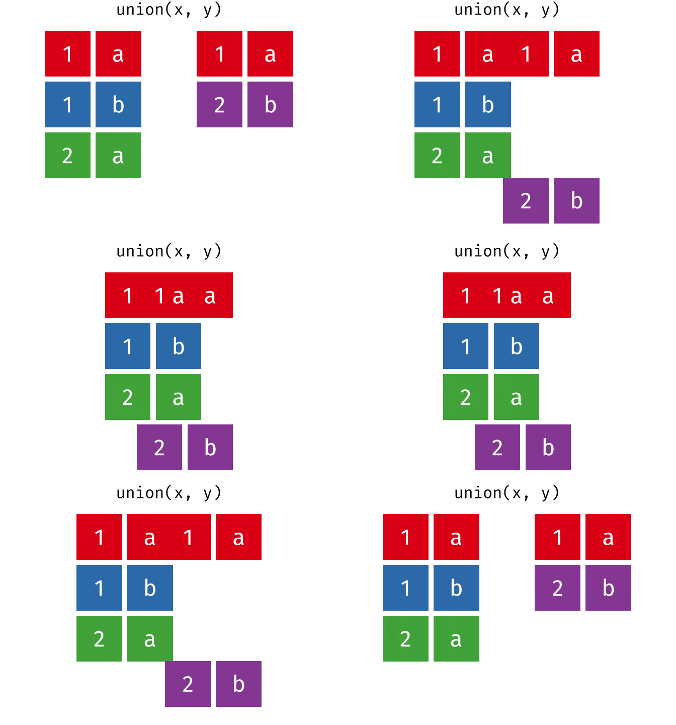
union()

union() returns all unique rows from both tables - the union set.

union(set_a, set_b)

# A tibble: 4 × 2
  city      country
  <chr>     <chr>  
1 Berlin    Germany
2 Hamburg   Germany
3 Munich    Germany
4 Frankfurt Germany

Hamburg and Munich appear in both tables but appear only once in the result.

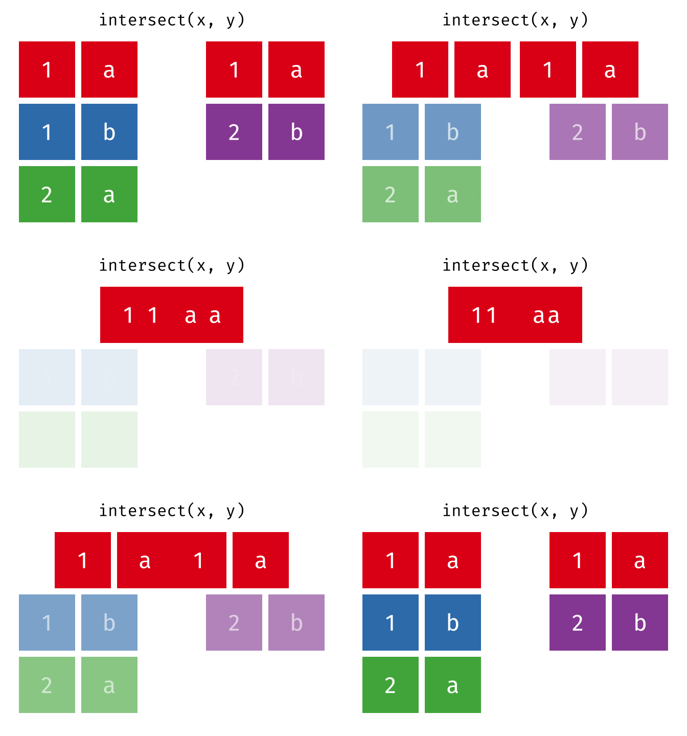
intersect()

intersect() returns only the rows that appear in both tables - the intersection.

intersect(set_a, set_b)

# A tibble: 2 × 2
  city    country
  <chr>   <chr>  
1 Hamburg Germany
2 Munich  Germany

Only Hamburg and Munich are in both tables.

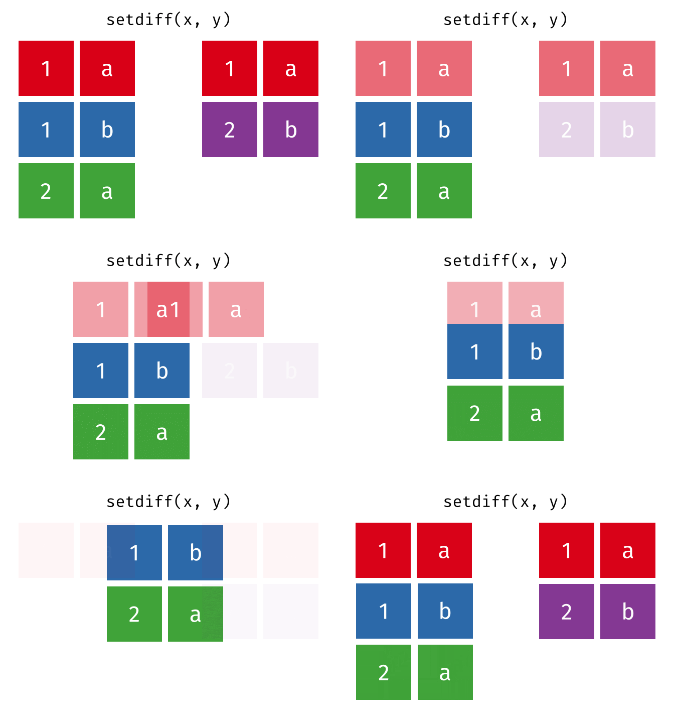
setdiff()

setdiff() returns the rows that are in the first but not in the second table - the difference set.

setdiff(set_a, set_b)

# A tibble: 1 × 2
  city   country
  <chr>  <chr>  
1 Berlin Germany

Berlin is only in set_a.

Note

With setdiff(), order matters! setdiff(a, b) and setdiff(b, a) return different results:

setdiff(set_b, set_a)

# A tibble: 1 × 2
  city      country
  <chr>     <chr>  
1 Frankfurt Germany

Frankfurt is only in set_b.

Reshaping Data (Wide ↔︎ Long)

Often we need to transform data between two formats:

Wide format: Each variable has its own column
Long format: Variable names become values in a column

Which format is “correct” depends on the use case. For many tidyverse functions and ggplot2, the long format is better suited, while the wide format is often more readable for humans.

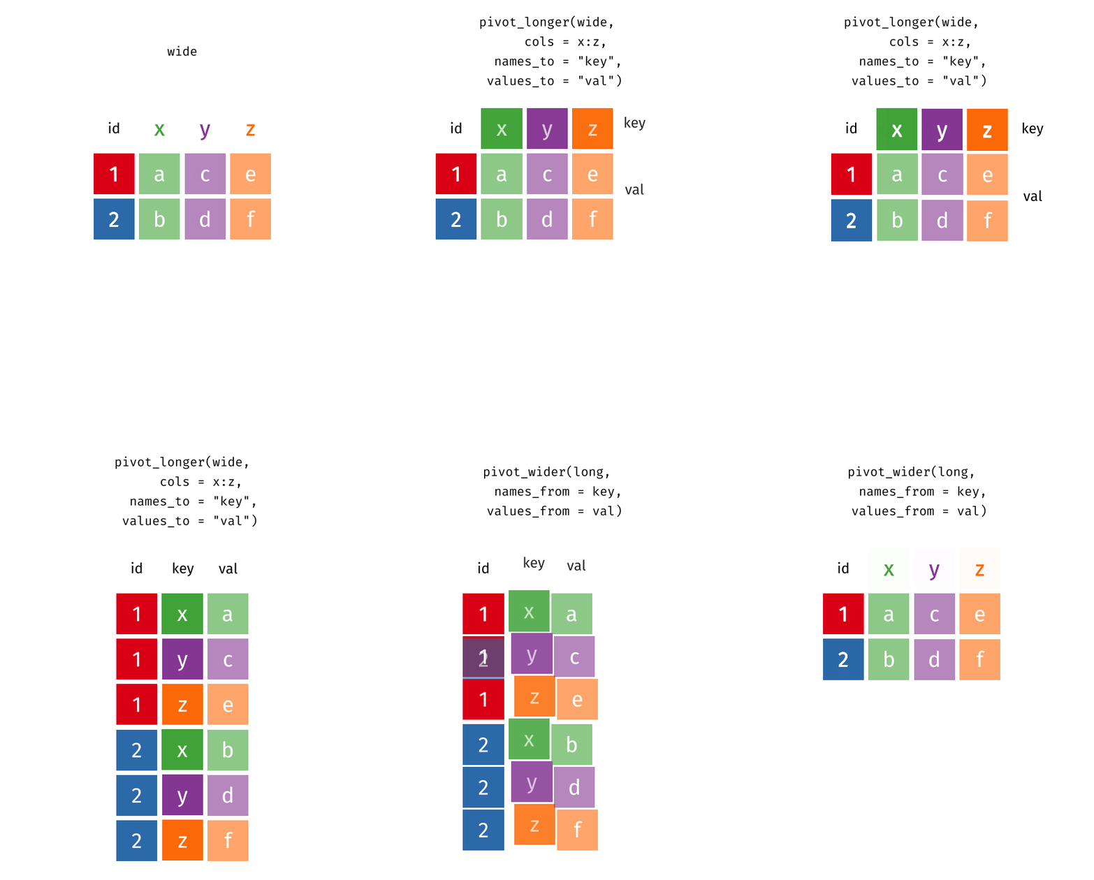
pivot_longer()

pivot_longer() transforms data from wide to long format - it makes the table “longer” (more rows, fewer columns).

Let’s look at cities_stats:

cities_stats

# A tibble: 10 × 3
   city        area_km2 green_space_pct
   <chr>          <dbl>           <dbl>
 1 Berlin           892            14.4
 2 Hamburg          755            16.8
 3 Munich           310            11.9
 4 Frankfurt        248            21.5
 5 Cologne          405            17.2
 6 Duesseldorf      217            18.9
 7 Stuttgart        207            24  
 8 Leipzig          297            14.8
 9 Dresden          328            12.3
10 Nuremberg        186            19.1

This is a typical wide format: each metric (area, green space) has its own column. For some analyses or visualizations, we want to convert this to long format:

cities_stats %>%
  pivot_longer(
    cols = c(area_km2, green_space_pct),
    names_to = "metric",
    values_to = "value"
  )

# A tibble: 20 × 3
   city        metric          value
   <chr>       <chr>           <dbl>
 1 Berlin      area_km2        892  
 2 Berlin      green_space_pct  14.4
 3 Hamburg     area_km2        755  
 4 Hamburg     green_space_pct  16.8
 5 Munich      area_km2        310  
 6 Munich      green_space_pct  11.9
 7 Frankfurt   area_km2        248  
 8 Frankfurt   green_space_pct  21.5
 9 Cologne     area_km2        405  
10 Cologne     green_space_pct  17.2
11 Duesseldorf area_km2        217  
12 Duesseldorf green_space_pct  18.9
13 Stuttgart   area_km2        207  
14 Stuttgart   green_space_pct  24  
15 Leipzig     area_km2        297  
16 Leipzig     green_space_pct  14.8
17 Dresden     area_km2        328  
18 Dresden     green_space_pct  12.3
19 Nuremberg   area_km2        186  
20 Nuremberg   green_space_pct  19.1

The key arguments:

cols: Which columns should be “collapsed”?
names_to: What should the new column be called that contains the old column names?
values_to: What should the new column be called that contains the values?

Now each city has two rows - one per metric. This is ideal for ggplot2 when you want to display both metrics in a faceted plot, for example.

Column Selection with Helper Functions

Instead of listing columns individually, you can use helper functions:

# All columns except "city"
cities_stats %>%
  pivot_longer(
    cols = -city,
    names_to = "metric",
    values_to = "value"
  )

# A tibble: 20 × 3
   city        metric          value
   <chr>       <chr>           <dbl>
 1 Berlin      area_km2        892  
 2 Berlin      green_space_pct  14.4
 3 Hamburg     area_km2        755  
 4 Hamburg     green_space_pct  16.8
 5 Munich      area_km2        310  
 6 Munich      green_space_pct  11.9
 7 Frankfurt   area_km2        248  
 8 Frankfurt   green_space_pct  21.5
 9 Cologne     area_km2        405  
10 Cologne     green_space_pct  17.2
11 Duesseldorf area_km2        217  
12 Duesseldorf green_space_pct  18.9
13 Stuttgart   area_km2        207  
14 Stuttgart   green_space_pct  24  
15 Leipzig     area_km2        297  
16 Leipzig     green_space_pct  14.8
17 Dresden     area_km2        328  
18 Dresden     green_space_pct  12.3
19 Nuremberg   area_km2        186  
20 Nuremberg   green_space_pct  19.1

# All numeric columns
cities_stats %>%
  pivot_longer(
    cols = where(is.numeric),
    names_to = "metric",
    values_to = "value"
  )

# A tibble: 20 × 3
   city        metric          value
   <chr>       <chr>           <dbl>
 1 Berlin      area_km2        892  
 2 Berlin      green_space_pct  14.4
 3 Hamburg     area_km2        755  
 4 Hamburg     green_space_pct  16.8
 5 Munich      area_km2        310  
 6 Munich      green_space_pct  11.9
 7 Frankfurt   area_km2        248  
 8 Frankfurt   green_space_pct  21.5
 9 Cologne     area_km2        405  
10 Cologne     green_space_pct  17.2
11 Duesseldorf area_km2        217  
12 Duesseldorf green_space_pct  18.9
13 Stuttgart   area_km2        207  
14 Stuttgart   green_space_pct  24  
15 Leipzig     area_km2        297  
16 Leipzig     green_space_pct  14.8
17 Dresden     area_km2        328  
18 Dresden     green_space_pct  12.3
19 Nuremberg   area_km2        186  
20 Nuremberg   green_space_pct  19.1

pivot_wider()

pivot_wider() is the inverse function: it transforms from long to wide format - the table becomes “wider” (fewer rows, more columns).

First, let’s create a long-format table:

cities_long <- cities_stats %>%
  pivot_longer(
    cols = -city,
    names_to = "metric",
    values_to = "value"
  )

cities_long

# A tibble: 20 × 3
   city        metric          value
   <chr>       <chr>           <dbl>
 1 Berlin      area_km2        892  
 2 Berlin      green_space_pct  14.4
 3 Hamburg     area_km2        755  
 4 Hamburg     green_space_pct  16.8
 5 Munich      area_km2        310  
 6 Munich      green_space_pct  11.9
 7 Frankfurt   area_km2        248  
 8 Frankfurt   green_space_pct  21.5
 9 Cologne     area_km2        405  
10 Cologne     green_space_pct  17.2
11 Duesseldorf area_km2        217  
12 Duesseldorf green_space_pct  18.9
13 Stuttgart   area_km2        207  
14 Stuttgart   green_space_pct  24  
15 Leipzig     area_km2        297  
16 Leipzig     green_space_pct  14.8
17 Dresden     area_km2        328  
18 Dresden     green_space_pct  12.3
19 Nuremberg   area_km2        186  
20 Nuremberg   green_space_pct  19.1

Now we transform back to wide format:

cities_long %>%
  pivot_wider(
    names_from = metric,
    values_from = value
  )

# A tibble: 10 × 3
   city        area_km2 green_space_pct
   <chr>          <dbl>           <dbl>
 1 Berlin           892            14.4
 2 Hamburg          755            16.8
 3 Munich           310            11.9
 4 Frankfurt        248            21.5
 5 Cologne          405            17.2
 6 Duesseldorf      217            18.9
 7 Stuttgart        207            24  
 8 Leipzig          297            14.8
 9 Dresden          328            12.3
10 Nuremberg        186            19.1

The key arguments:

names_from: Which column contains the future column names?
values_from: Which column contains the values?

Alternative Function Names in Other Packages

You may have already used other functions in this context. Here are some alternatives, some of which are now deprecated:

melt() & dcast() from {data.table}
fold() & unfold() from {databases}
melt() & cast() from {reshape}
melt() & dcast() from {reshape2}
unpivot() & pivot() from {spreadsheets}
gather() & spread() from {tidyr} < v1.0.0

Typical Use Case: Cross Tables

pivot_wider() is also useful for creating cross tables. Suppose we have sales data:

sales <- tibble(
  product = c("Apple", "Apple", "Pear", "Pear"),
  quarter = c("Q1", "Q2", "Q1", "Q2"),
  revenue = c(100, 120, 80, 90)
)

sales

# A tibble: 4 × 3
  product quarter revenue
  <chr>   <chr>     <dbl>
1 Apple   Q1          100
2 Apple   Q2          120
3 Pear    Q1           80
4 Pear    Q2           90

sales %>%
  pivot_wider(
    names_from = quarter,
    values_from = revenue
  )

# A tibble: 2 × 3
  product    Q1    Q2
  <chr>   <dbl> <dbl>
1 Apple     100   120
2 Pear       80    90

Now we have a clear cross table with products in rows and quarters in columns.

Exercise: Pivoting Workflow

First prepare a dataset in long format:

# Simulate PlantGrowth with multiple measurements
set.seed(42)
plants_long <- PlantGrowth %>%
  mutate(
    plant_id = 1:n(),
    height_cm = weight * 5 + rnorm(n(), mean = 0, sd = 2)
  ) %>%
  pivot_longer(
    cols = c(weight, height_cm),
    names_to = "measurement",
    values_to = "value"
  ) %>%
  select(plant_id, group, measurement, value)

plants_long

# A tibble: 60 × 4
   plant_id group measurement value
      <int> <fct> <chr>       <dbl>
 1        1 ctrl  weight       4.17
 2        1 ctrl  height_cm   23.6 
 3        2 ctrl  weight       5.58
 4        2 ctrl  height_cm   26.8 
 5        3 ctrl  weight       5.18
 6        3 ctrl  height_cm   26.6 
 7        4 ctrl  weight       6.11
 8        4 ctrl  height_cm   31.8 
 9        5 ctrl  weight       4.5 
10        5 ctrl  height_cm   23.3 
# ℹ 50 more rows

Exercise

Perform the following transformations:

Transform plants_long to wide format so that weight and height_cm each have their own columns.
Add a new column bmi (Body Mass Index for plants) that calculates the ratio weight / height_cm.
Transform the dataset back to long format so that all three variables (weight, height_cm, and bmi) appear in the measurement column.

Solution

# a) Create wide format
plants_wide <- plants_long %>%
  pivot_wider(
    names_from = measurement,
    values_from = value
  )

plants_wide

# A tibble: 30 × 4
   plant_id group weight height_cm
      <int> <fct>  <dbl>     <dbl>
 1        1 ctrl    4.17      23.6
 2        2 ctrl    5.58      26.8
 3        3 ctrl    5.18      26.6
 4        4 ctrl    6.11      31.8
 5        5 ctrl    4.5       23.3
 6        6 ctrl    4.61      22.8
 7        7 ctrl    5.17      28.9
 8        8 ctrl    4.53      22.5
 9        9 ctrl    5.33      30.7
10       10 ctrl    5.14      25.6
# ℹ 20 more rows

# b) Add new column
plants_wide <- plants_wide %>%
  mutate(bmi = weight / height_cm)

plants_wide

# A tibble: 30 × 5
   plant_id group weight height_cm   bmi
      <int> <fct>  <dbl>     <dbl> <dbl>
 1        1 ctrl    4.17      23.6 0.177
 2        2 ctrl    5.58      26.8 0.208
 3        3 ctrl    5.18      26.6 0.195
 4        4 ctrl    6.11      31.8 0.192
 5        5 ctrl    4.5       23.3 0.193
 6        6 ctrl    4.61      22.8 0.202
 7        7 ctrl    5.17      28.9 0.179
 8        8 ctrl    4.53      22.5 0.202
 9        9 ctrl    5.33      30.7 0.174
10       10 ctrl    5.14      25.6 0.201
# ℹ 20 more rows

# c) Back to long format (all three variables)
plants_final_long <- plants_wide %>%
  pivot_longer(
    cols = c(weight, height_cm, bmi),
    names_to = "measurement",
    values_to = "value"
  )

plants_final_long

# A tibble: 90 × 4
   plant_id group measurement  value
      <int> <fct> <chr>        <dbl>
 1        1 ctrl  weight       4.17 
 2        1 ctrl  height_cm   23.6  
 3        1 ctrl  bmi          0.177
 4        2 ctrl  weight       5.58 
 5        2 ctrl  height_cm   26.8  
 6        2 ctrl  bmi          0.208
 7        3 ctrl  weight       5.18 
 8        3 ctrl  height_cm   26.6  
 9        3 ctrl  bmi          0.195
10        4 ctrl  weight       6.11 
# ℹ 80 more rows

Summary

Well done! You now master the most important techniques for combining and reshaping tables in R.

Key Takeaways

Stacking Tables:
- bind_rows(): Stack rows vertically - works even with different columns (missing ones are filled with NA)
- bind_cols(): Glue columns horizontally - Caution: no intelligent linking, order must match!
Mutating Joins (add columns):
- left_join(): Keep all rows from the left table - the default case
- right_join(): Keep all rows from the right table
- inner_join(): Only rows with a partner in both tables
- full_join(): All rows from both tables
Filtering Joins (only filter, no new columns):
- semi_join(): Rows from x that have a partner in y
- anti_join(): Rows from x that have no partner in y - ideal for “What’s missing?” questions
Set Operations (tables as sets, require identical columns):
- union(): All unique rows from both
- intersect(): Only rows that appear in both
- setdiff(): Rows from x that are not in y
Pivoting (change data format):
- pivot_longer(): Wide → Long (more rows, fewer columns)
- pivot_wider(): Long → Wide (fewer rows, more columns)
Best Practices:
- For different column names: by = c("name_left" = "name_right")
- When in doubt, use left_join() instead of bind_cols()
- Use anti_join() for data quality checks

Citation

BibTeX citation:

@online{schmidt2026,
  author = {{Dr. Paul Schmidt}},
  publisher = {BioMath GmbH},
  title = {1. {Combining} {Tables}},
  date = {2026-02-07},
  url = {https://biomathcontent.netlify.app/content/r_more/01_joins.html},
  langid = {en}
}

For attribution, please cite this work as:

Dr. Paul Schmidt. 2026. “1. Combining Tables.” BioMath GmbH. February 7, 2026. https://biomathcontent.netlify.app/content/r_more/01_joins.html.