5. Factors

To install and load all packages used in this chapter, run the following code:

for (pkg in c("forcats", "janitor", "patchwork", "tidyverse")) {
  if (!require(pkg, character.only = TRUE)) install.packages(pkg)
}

library(forcats)
library(janitor)
library(patchwork)
library(tidyverse)

Introduction

Anyone working with categorical data in R will sooner or later encounter the concept of factors. For beginners, they are often confusing: Why does a column suddenly behave differently than expected? Why do the bars in the chart appear in a strange order?

This chapter explains what factors are, when you need them, and how to elegantly manipulate them with the {forcats} package.

Example Data

We again use the starwars dataset, filtered to humans:

humans <- starwars %>%
  filter(species == "Human") %>%
  select(name, height, mass, hair_color, eye_color, gender)

humans

# A tibble: 35 × 6
   name               height  mass hair_color    eye_color gender   
   <chr>               <int> <dbl> <chr>         <chr>     <chr>    
 1 Luke Skywalker        172    77 blond         blue      masculine
 2 Darth Vader           202   136 none          yellow    masculine
 3 Leia Organa           150    49 brown         brown     feminine 
 4 Owen Lars             178   120 brown, grey   blue      masculine
 5 Beru Whitesun Lars    165    75 brown         blue      feminine 
 6 Biggs Darklighter     183    84 black         brown     masculine
 7 Obi-Wan Kenobi        182    77 auburn, white blue-gray masculine
 8 Anakin Skywalker      188    84 blond         blue      masculine
 9 Wilhuff Tarkin        180    NA auburn, grey  blue      masculine
10 Han Solo              180    80 brown         brown     masculine
# ℹ 25 more rows

Character vs. Factor: The Difference

Character: Simply Text

A character variable is simply text. R treats each value as an independent string:

# eye_color is a character vector
class(humans$eye_color)

[1] "character"

# Unique values (in order of first occurrence)
unique(humans$eye_color)

[1] "blue"      "yellow"    "brown"     "blue-gray" "hazel"     "dark"     
[7] "unknown"  

When we sort character values, it happens alphabetically:

sort(unique(humans$eye_color))

[1] "blue"      "blue-gray" "brown"     "dark"      "hazel"     "unknown"  
[7] "yellow"   

Factor: Text with Structure

A factor is text plus additional information:

1. Levels: The possible categories
2. Order: The sorting of the levels

# Convert character to factor
eye_factor <- factor(humans$eye_color)

class(eye_factor)

[1] "factor"

levels(eye_factor)  # The stored levels

[1] "blue"      "blue-gray" "brown"     "dark"      "hazel"     "unknown"  
[7] "yellow"   

The levels are sorted alphabetically by default. But we can define a custom order:

eye_custom <- factor(
  humans$eye_color,
  levels = c("blue", "brown", "hazel", "dark", "blue-gray")
)

levels(eye_custom)

[1] "blue"      "brown"     "hazel"     "dark"      "blue-gray"

Why Does This Matter?

The level order affects:

• Sorting in tables
• Order in graphics (e.g., bar charts)
• Reference category in statistical models

# With character: alphabetical order
p1 <- humans %>%
  count(eye_color) %>%
  ggplot(aes(x = eye_color, y = n)) +
  geom_col() +
  labs(title = "Character: alphabetical") +
  theme_minimal()

# With factor: our order
p2 <- humans %>%
  mutate(eye_color = factor(eye_color,
                            levels = c("brown", "blue", "hazel", "dark", "blue-gray"))) %>%
  count(eye_color) %>%
  ggplot(aes(x = eye_color, y = n)) +
  geom_col() +
  labs(title = "Factor: custom order") +
  theme_minimal()

# Display side by side
p1 + p2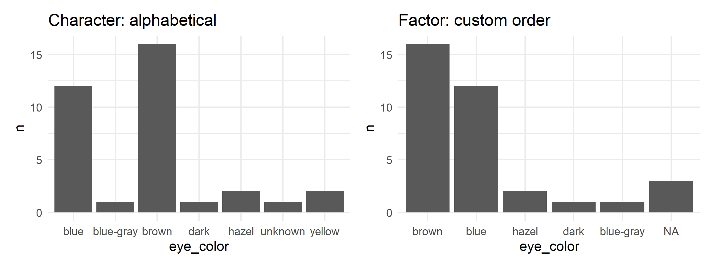

TipExercise: Character vs. Factor

a) Check with class() whether hair_color in the humans dataset is a character or factor.

b) Convert hair_color to a factor and display the levels.

c) Create a factor for hair_color with the order: “brown”, “black”, “blond”, “auburn”, then all others.

NoteSolution

# a) Check class
class(humans$hair_color)

[1] "character"

# b) Convert to factor
hair_factor <- factor(humans$hair_color)
levels(hair_factor)

 [1] "auburn"        "auburn, grey"  "auburn, white" "black"        
 [5] "blond"         "brown"         "brown, grey"   "grey"         
 [9] "none"          "white"        

# c) With custom order
hair_custom <- factor(
  humans$hair_color,
  levels = c("brown", "black", "blond", "auburn",
             "auburn, grey", "auburn, white", "grey", "white", "none")
)
levels(hair_custom)

[1] "brown"         "black"         "blond"         "auburn"       
[5] "auburn, grey"  "auburn, white" "grey"          "white"        
[9] "none"         

Creating Factors

factor() vs. as_factor()

There are two main functions for creating factors:

colors <- c("red", "blue", "red", "green", "blue")

# factor(): Levels alphabetical
factor(colors)

[1] red   blue  red   green blue 
Levels: blue green red

# as_factor(): Levels by order of first occurrence
as_factor(colors)

[1] red   blue  red   green blue 
Levels: red blue green

Function	Package	Level Order
factor()	base R	Alphabetical
as_factor()	forcats	By occurrence in vector

as_factor() is often more practical because the order of the data is preserved.

Specifying Levels Explicitly

With the levels argument, we can determine the order ourselves:

# Custom order
satisfaction <- c("medium", "high", "low", "high", "medium")

# WRONG: alphabetical
factor(satisfaction)

[1] medium high   low    high   medium
Levels: high low medium

# RIGHT: logical order
factor(satisfaction, levels = c("low", "medium", "high"))

[1] medium high   low    high   medium
Levels: low medium high

forcats: Manipulating Factors

The {forcats} package (part of the tidyverse) provides practical functions for factor manipulation. All functions start with fct_.

Changing Order

fct_relevel() – Manual Reordering

# Original order
humans %>%
  mutate(eye_color = factor(eye_color)) %>%
  pull(eye_color) %>%
  levels()

[1] "blue"      "blue-gray" "brown"     "dark"      "hazel"     "unknown"  
[7] "yellow"   

# Move "brown" to the beginning
humans %>%
  mutate(eye_color = fct_relevel(eye_color, "brown")) %>%
  pull(eye_color) %>%
  levels()

[1] "brown"     "blue"      "blue-gray" "dark"      "hazel"     "unknown"  
[7] "yellow"   

# Multiple levels in specific order
humans %>%
  mutate(eye_color = fct_relevel(eye_color, "brown", "blue", "hazel")) %>%
  pull(eye_color) %>%
  levels()

[1] "brown"     "blue"      "hazel"     "blue-gray" "dark"      "unknown"  
[7] "yellow"   

fct_reorder() – Sort by Another Variable

Particularly useful for graphics – sort categories by a numerical value:

# Average height by hair color
hair_height <- humans %>%
  filter(!is.na(hair_color), !is.na(height)) %>%
  group_by(hair_color) %>%
  summarise(mean_height = mean(height), n = n()) %>%
  filter(n >= 2)  # Only groups with at least 2 people

# Without fct_reorder: alphabetical
p1 <- hair_height %>%
  ggplot(aes(x = hair_color, y = mean_height)) +
  geom_col() +
  labs(title = "Alphabetical") +
  theme_minimal() +
  theme(axis.text.x = element_text(angle = 45, hjust = 1))

# With fct_reorder: sorted by height
p2 <- hair_height %>%
  ggplot(aes(x = fct_reorder(hair_color, mean_height), y = mean_height)) +
  geom_col() +
  labs(title = "Sorted by height", x = "hair_color") +
  theme_minimal() +
  theme(axis.text.x = element_text(angle = 45, hjust = 1))

p1 + p2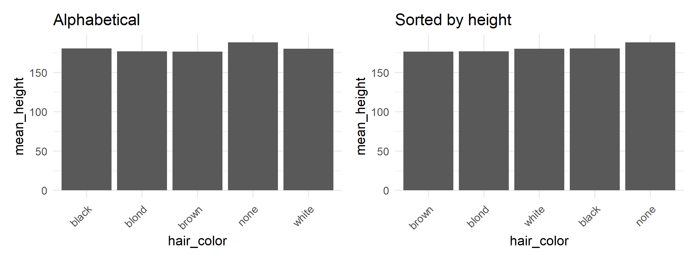

fct_infreq() – Sort by Frequency

humans %>%
  mutate(eye_color = fct_infreq(eye_color)) %>%
  pull(eye_color) %>%
  levels()

[1] "brown"     "blue"      "hazel"     "yellow"    "blue-gray" "dark"     
[7] "unknown"  

The most frequent categories come first – ideal for bar charts.

fct_rev() – Reverse Order

# Most frequent first, then reverse (least frequent first)
humans %>%
  mutate(eye_color = fct_rev(fct_infreq(eye_color))) %>%
  pull(eye_color) %>%
  levels()

[1] "unknown"   "dark"      "blue-gray" "yellow"    "hazel"     "blue"     
[7] "brown"    

Combining Levels

fct_lump_n() – Combine Rare into “Other”

# Keep only the 3 most frequent, rest becomes "Other"
humans %>%
  mutate(eye_color = fct_lump_n(eye_color, n = 3)) %>%
  tabyl(eye_color)

 eye_color  n    percent
      blue 12 0.34285714
     brown 16 0.45714286
     hazel  2 0.05714286
    yellow  2 0.05714286
     Other  3 0.08571429

# With custom label
humans %>%
  mutate(eye_color = fct_lump_n(eye_color, n = 3, other_level = "Misc")) %>%
  tabyl(eye_color)

 eye_color  n    percent
      blue 12 0.34285714
     brown 16 0.45714286
     hazel  2 0.05714286
    yellow  2 0.05714286
      Misc  3 0.08571429

Related functions:

• fct_lump_min() – Combine if fewer than n occurrences
• fct_lump_prop() – Combine if proportion below x%

fct_collapse() – Combine Multiple Levels

humans %>%
  mutate(
    eye_group = fct_collapse(
      eye_color,
      "light" = c("blue", "blue-gray", "hazel"),
      "dark" = c("brown", "dark")
    )
  ) %>%
  tabyl(eye_group)

 eye_group  n    percent
     light 15 0.42857143
      dark 17 0.48571429
   unknown  1 0.02857143
    yellow  2 0.05714286

Renaming Levels

fct_recode()

humans %>%
  mutate(
    eye_color_full = fct_recode(
      eye_color,
      "Blue" = "blue",
      "Brown" = "brown",
      "Dark" = "dark",
      "Hazel" = "hazel",
      "Blue-Gray" = "blue-gray"
    )
  ) %>%
  tabyl(eye_color_full)

 eye_color_full  n    percent
           Blue 12 0.34285714
      Blue-Gray  1 0.02857143
          Brown 16 0.45714286
           Dark  1 0.02857143
          Hazel  2 0.05714286
        unknown  1 0.02857143
         yellow  2 0.05714286

TipExercise: forcats

Work with the humans dataset:

a) Create a bar chart of hair_color where the bars are sorted by frequency (most frequent on the left).

b) Combine all hair colors except the 3 most frequent under “Other” and create a frequency table with tabyl().

c) Rename the levels of gender: “feminine” → “female”, “masculine” → “male”.

NoteSolution

# a) Bar chart by frequency
humans %>%
  filter(!is.na(hair_color)) %>%
  ggplot(aes(x = fct_infreq(hair_color))) +
  geom_bar() +
  labs(x = "Hair color", y = "Count") +
  theme_minimal() +
  theme(axis.text.x = element_text(angle = 45, hjust = 1))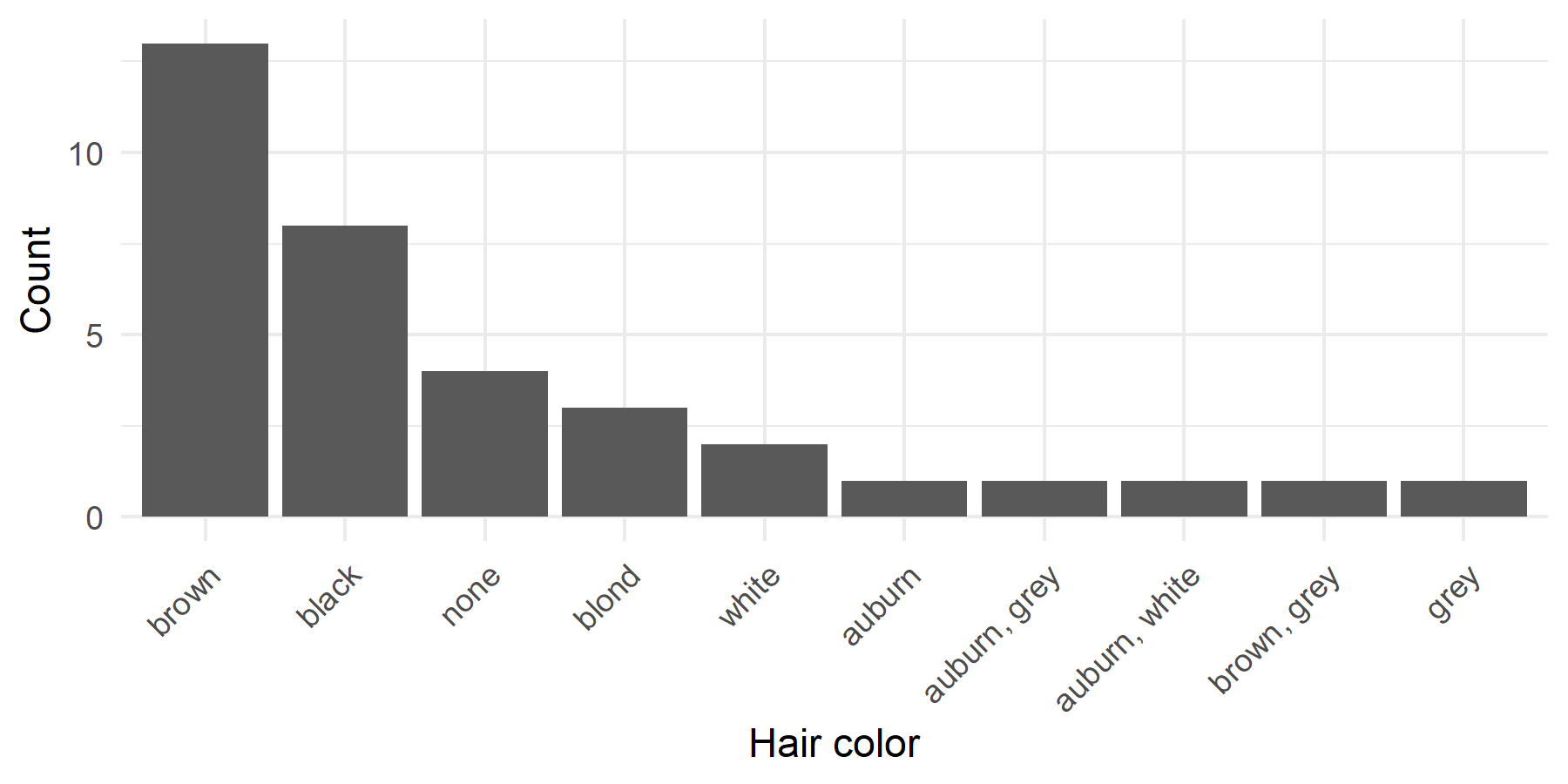

# b) Lump and tabyl
humans %>%
  mutate(hair_color = fct_lump_n(hair_color, n = 3, other_level = "Other")) %>%
  tabyl(hair_color, show_na = FALSE)

 hair_color  n   percent
      black  8 0.2285714
      brown 13 0.3714286
       none  4 0.1142857
      Other 10 0.2857143

# c) Rename gender
humans %>%
  mutate(
    gender_renamed = fct_recode(
      gender,
      "female" = "feminine",
      "male" = "masculine"
    )
  ) %>%
  tabyl(gender_renamed)

 gender_renamed  n   percent
         female  9 0.2571429
           male 26 0.7428571

Practical Applications

Factors in ggplot2

The level order determines the arrangement in graphics:

# Sensible order for bar chart
humans %>%
  filter(!is.na(eye_color)) %>%
  mutate(eye_color = fct_infreq(eye_color)) %>%  # By frequency
  ggplot(aes(x = eye_color, fill = eye_color)) +
  geom_bar() +
  coord_flip() +  # Horizontal bars
  labs(
    title = "Eye Colors of Star Wars Humans",
    x = NULL,
    y = "Count"
  ) +
  theme_minimal() +
  theme(legend.position = "none")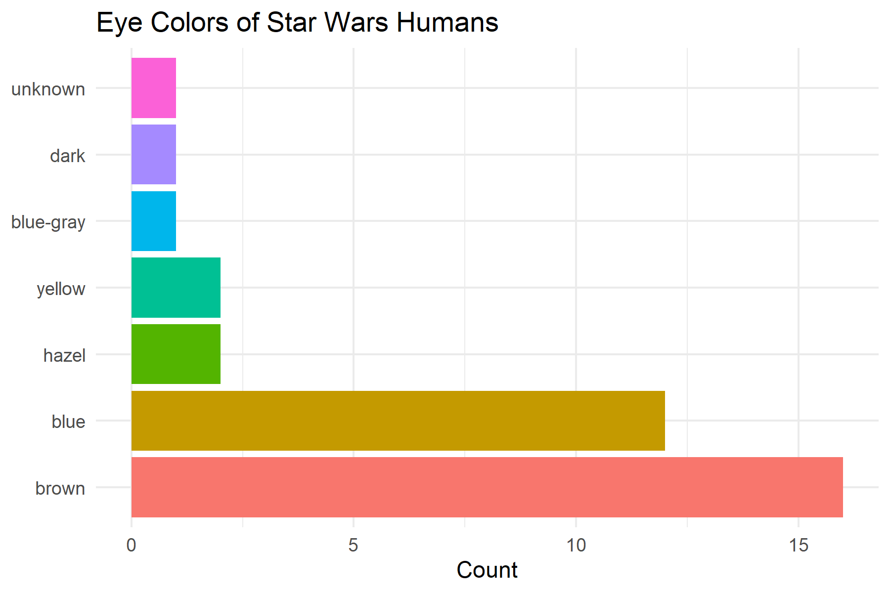

With horizontal bar charts, you often want the most frequent category at the top. For this, combine fct_infreq() with fct_rev():

humans %>%
  filter(!is.na(eye_color)) %>%
  mutate(eye_color = fct_rev(fct_infreq(eye_color))) %>%  # Reversed
  ggplot(aes(x = eye_color, fill = eye_color)) +
  geom_bar() +
  coord_flip() +
  labs(
    title = "Most Frequent Category on Top",
    x = NULL,
    y = "Count"
  ) +
  theme_minimal() +
  theme(legend.position = "none")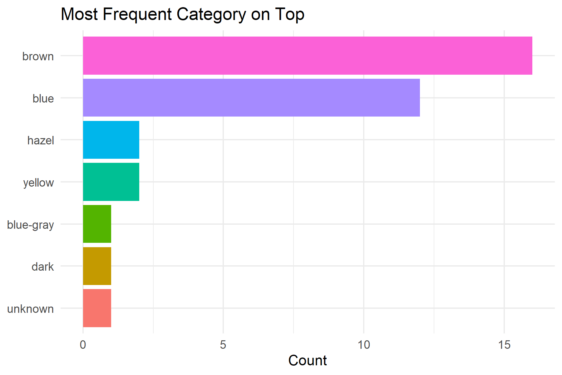

Factors in tabyl()

tabyl() also respects the level order:

# Without factor: alphabetical
humans %>%
  tabyl(eye_color)

 eye_color  n    percent
      blue 12 0.34285714
 blue-gray  1 0.02857143
     brown 16 0.45714286
      dark  1 0.02857143
     hazel  2 0.05714286
   unknown  1 0.02857143
    yellow  2 0.05714286

# With factor: by our order
humans %>%
  mutate(eye_color = fct_relevel(eye_color, "brown", "blue")) %>%
  tabyl(eye_color)

 eye_color  n    percent
     brown 16 0.45714286
      blue 12 0.34285714
 blue-gray  1 0.02857143
      dark  1 0.02857143
     hazel  2 0.05714286
   unknown  1 0.02857143
    yellow  2 0.05714286

# By frequency
humans %>%
  mutate(eye_color = fct_infreq(eye_color)) %>%
  tabyl(eye_color)

 eye_color  n    percent
     brown 16 0.45714286
      blue 12 0.34285714
     hazel  2 0.05714286
    yellow  2 0.05714286
 blue-gray  1 0.02857143
      dark  1 0.02857143
   unknown  1 0.02857143

This is particularly useful for reports where the order of categories should have a substantive meaning (e.g., “excellent”, “good”, “satisfactory”, “poor”).

Summary

Factors are more powerful than simple character variables because they store a defined set of categories with a specific order.

NoteKey Takeaways

Character vs. Factor:

Aspect	Character	Factor
Stores	Only text	Text + levels + order
Sorting	Alphabetical	By level order
Unknown values	Allowed	Become NA (if not in levels)
Use case	Free text	Categories with fixed values

When Character, When Factor?

• Character: Free text, names, IDs, comments
• Factor: Categories with defined values (gender, Likert scales, regions)

Key forcats Functions:

Function	Purpose
fct_relevel()	Manually reorder levels
fct_reorder()	Sort by numerical variable
fct_infreq()	Sort by frequency
fct_rev()	Reverse order
fct_lump_n()	Combine rare into “Other”
fct_collapse()	Combine multiple levels
fct_recode()	Rename levels

Typical Workflow for Graphics:

data %>%
  mutate(category = fct_infreq(category)) %>%  # By frequency
  ggplot(aes(x = category)) +
  geom_bar()

Further Resources:

• forcats Documentation
• R for Data Science: Factors