| person_id | Q1_apple | Q1_banana | Q1_cherry | Q1_mango | Q1_orange |
|---|---|---|---|---|---|
| 1 | 1 | 0 | 1 | 0 | 1 |
| 2 | 0 | 1 | 0 | 0 | 0 |
| 3 | 1 | 1 | 1 | 1 | 1 |
| 4 | 1 | 0 | 1 | 1 | 0 |
What Are Multiple Response Questions?
Many surveys and interviews include questions where respondents can select not just one, but multiple answer options. A classic example would be the question “Which of these fruits do you like?” with five options. Unlike a single-choice question, where exactly one option must be selected, respondents can check any number of options here - from none at all to all five.
This seemingly simple extension has far-reaching consequences for data structure and analysis: While single-choice only requires one column with the selected categories, multiple-choice needs different approaches. Let’s imagine four people answering our fruit question:
Which of these fruits do you like?
Person 1
☑ Apple
☐ Banana
☑ Cherry
☐ Mango
☑ Orange
Person 2
☐ Apple
☑ Banana
☐ Cherry
☐ Mango
☐ Orange
Person 3
☑ Apple
☑ Banana
☑ Cherry
☑ Mango
☑ Orange
Person 4
☑ Apple
☐ Banana
☑ Cherry
☑ Mango
☐ Orange
Person 1 likes three fruits, Person 2 only one, Person 3 all five, and Person 4 three again. How do we store this information in a table? There are different formats for this.
Data Formats for Multiple Responses
Dichotomous Format (Wide)
The most common format in practice: Each answer option becomes its own column with values 0 (not selected) and 1 (selected). This makes the table “wide”, which is why it’s also called the wide format.
This format is typical for exports from survey tools like Google Forms, SurveyMonkey, Qualtrics, LimeSurvey, or REDCap. The related columns of a multiple response question often share a common prefix (here: Q1_), which makes it easier to identify and select the columns. The advantage: Each row is one person, and you can immediately see which combinations were selected. The disadvantage: With many answer options, the table becomes very wide.
Collapsed Format (Delimited)
A more compact alternative: All selected options are in a single column, separated by a delimiter such as semicolon, comma, or pipe.
| person_id | Q1_fruit |
|---|---|
| 1 | Apple; Cherry; Orange |
| 2 | Banana |
| 3 | Apple; Banana; Cherry; Mango; Orange |
| 4 | Apple; Cherry; Mango |
This format often arises from manual data entry in Excel or from older database systems. It’s space-saving and human-readable, but must first be converted to another format for statistical analysis.
Long Format
In the long format, there is one row per selected option. This means: A person who selected three fruits appears in three rows.
| person_id | fruit |
|---|---|
| 1 | Apple |
| 1 | Cherry |
| 1 | Orange |
| 2 | Banana |
| 3 | Apple |
| 3 | Banana |
| 3 | Cherry |
| 3 | Mango |
| 3 | Orange |
| 4 | Apple |
| 4 | Cherry |
| 4 | Mango |
The long format is typical for relational databases and particularly well-suited for analysis with tidyverse functions like count() or group_by(). The disadvantage: The table becomes very long with many responses, and people who selected nothing don’t appear at all.
NoteFor SPSS Users: Multiple Response Sets
In SPSS, multiple responses must be analyzed through a special mechanism: You first define a “Multiple Response Set” from the individual variables before you can calculate frequencies. SPSS distinguishes between counting “by cases” (percent of respondents) and “by responses” (percent of all given responses).
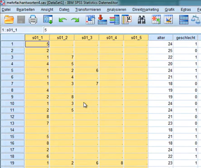
In R, this detour via set definitions is not necessary - we work directly with the data in one of the three formats. Those who still prefer SPSS-like syntax can use the R packages expss (with mrset() and tab_stat_cpct()) or sjmisc (with frq() and flat_table()).
A detailed guide to the SPSS approach is shown in this video (in German): Multiple Responses in SPSS
Converting Between Formats
In practice, you often receive data in one format but want to analyze it in another. With tidyverse functions, any format can be converted to any other. Let’s first define our three example datasets explicitly:
# Dichotomous Format (Wide)
fruit_dichotom <- tibble(
  person_id = 1:4,
  Q1_apple  = c(1, 0, 1, 1),
  Q1_banana = c(0, 1, 1, 0),
  Q1_cherry = c(1, 0, 1, 1),
  Q1_mango  = c(0, 0, 1, 1),
  Q1_orange = c(1, 0, 1, 0)
)

# Collapsed Format
fruit_collapsed <- tibble(
  person_id = 1:4,
  Q1_fruit = c("Apple; Cherry; Orange",
               "Banana",
               "Apple; Banana; Cherry; Mango; Orange",
               "Apple; Cherry; Mango")
)

# Long Format
fruit_long <- tibble(
  person_id = c(1, 1, 1, 2, 3, 3, 3, 3, 3, 4, 4, 4),
  fruit = c("Apple", "Cherry", "Orange",
            "Banana",
            "Apple", "Banana", "Cherry", "Mango", "Orange",
            "Apple", "Cherry", "Mango")
)
Dichotomous to Long
The dichotomous format is converted to long format using pivot_longer(). The common prefix Q1_ allows selecting the related columns with starts_with(). Then we filter only the rows where an option was selected (value = 1).
fruit_dichotom %>%
  pivot_longer(
    cols = starts_with("Q1_"),       # all columns with prefix Q1_
    names_to = "fruit",              # column names become values
    names_prefix = "Q1_",            # remove prefix
    values_to = "selected"           # 0/1 values in new column
  ) %>%
  filter(selected == 1) %>%          # keep only selected options
  select(-selected)                  # remove helper column
# A tibble: 12 × 2
person_id fruit
<int> <chr>
1 1 apple
2 1 cherry
3 1 orange
4 2 banana
5 3 apple
6 3 banana
7 3 cherry
8 3 mango
9 3 orange
10 4 apple
11 4 cherry
12 4 mango Dichotomous to Collapsed
For conversion to collapsed format, we first pivot to long format, filter the selected options, and then combine them with summarise() and str_c().
fruit_dichotom %>%
  pivot_longer(
    cols = starts_with("Q1_"),
    names_to = "fruit",
    names_prefix = "Q1_",
    values_to = "selected"
  ) %>%
  filter(selected == 1) %>%
  summarise(
    Q1_fruit = str_c(str_to_title(fruit), collapse = "; "),
    .by = person_id
  )
# A tibble: 4 × 2
person_id Q1_fruit
<int> <chr>
1 1 Apple; Cherry; Orange
2 2 Banana
3 3 Apple; Banana; Cherry; Mango; Orange
4 4 Apple; Cherry; Mango Long to Dichotomous
The reverse direction: We add a helper column with value 1 and then pivot to wide format with pivot_wider(). Missing values are filled with 0.
fruit_long %>%
  mutate(
    fruit = str_to_lower(fruit),     # consistent spelling
    selected = 1                     # helper column
  ) %>%
  pivot_wider(
    names_from = fruit,
    names_prefix = "Q1_",            # add prefix
    values_from = selected,
    values_fill = 0                  # not selected = 0
  )
# A tibble: 4 × 6
person_id Q1_apple Q1_cherry Q1_orange Q1_banana Q1_mango
<dbl> <dbl> <dbl> <dbl> <dbl> <dbl>
1 1 1 1 1 0 0
2 2 0 0 0 1 0
3 3 1 1 1 1 1
4 4 1 1 0 0 1Long to Collapsed
In long format, we group by person and concatenate the fruits into a string.
fruit_long %>%
  summarise(
    Q1_fruit = str_c(fruit, collapse = "; "),
    .by = person_id
  )
# A tibble: 4 × 2
person_id Q1_fruit
<dbl> <chr>
1 1 Apple; Cherry; Orange
2 2 Banana
3 3 Apple; Banana; Cherry; Mango; Orange
4 4 Apple; Cherry; Mango Collapsed to Long
The collapsed format is split using separate_longer_delim(). This function creates a separate row for each value between the delimiters.
fruit_collapsed %>%
  separate_longer_delim(Q1_fruit, delim = "; ") %>%
  rename(fruit = Q1_fruit) %>%       # rename column
  mutate(fruit = str_trim(fruit))    # remove any whitespace
# A tibble: 12 × 2
person_id fruit
<int> <chr>
1 1 Apple
2 1 Cherry
3 1 Orange
4 2 Banana
5 3 Apple
6 3 Banana
7 3 Cherry
8 3 Mango
9 3 Orange
10 4 Apple
11 4 Cherry
12 4 Mango Collapsed to Dichotomous
For conversion to dichotomous format, we take the detour via long format.
fruit_collapsed %>%
  separate_longer_delim(Q1_fruit, delim = "; ") %>%
  mutate(
    fruit = str_to_lower(str_trim(Q1_fruit)),
    selected = 1
  ) %>%
  select(-Q1_fruit) %>%
  pivot_wider(
    names_from = fruit,
    names_prefix = "Q1_",
    values_from = selected,
    values_fill = 0
  )
# A tibble: 4 × 6
person_id Q1_apple Q1_cherry Q1_orange Q1_banana Q1_mango
<int> <dbl> <dbl> <dbl> <dbl> <dbl>
1 1 1 1 1 0 0
2 2 0 0 0 1 0
3 3 1 1 1 1 1
4 4 1 1 0 0 1Analysis: Frequencies
For the previous examples, we used a minimal dataset with only four people to demonstrate the formats clearly. For a realistic analysis, we now work with a larger dataset: 20 respondents (8 male, 12 female) answered the same fruit question.
# Larger dataset in dichotomous format
survey <- tibble(
  person_id = 1:20,
  gender = c("m", "f", "f", "m", "f", "m", "f", "f", "m", "f",
             "f", "m", "f", "m", "f", "m", "f", "f", "m", "f"),
  Q1_apple  = c(1, 1, 0, 1, 1, 0, 1, 1, 1, 0, 1, 1, 0, 1, 1, 0, 1, 1, 0, 1),
  Q1_banana = c(0, 1, 1, 0, 1, 1, 1, 1, 0, 1, 1, 0, 1, 0, 1, 1, 0, 1, 1, 0),
  Q1_cherry = c(1, 1, 1, 0, 1, 0, 1, 0, 1, 1, 1, 0, 1, 1, 0, 1, 1, 0, 1, 1),
  Q1_mango  = c(0, 0, 1, 1, 0, 0, 1, 0, 0, 1, 0, 1, 0, 0, 1, 0, 1, 0, 0, 1),
  Q1_orange = c(1, 0, 0, 1, 0, 1, 1, 1, 1, 0, 0, 1, 0, 1, 0, 0, 0, 1, 0, 0)
)

survey
# A tibble: 20 × 7
person_id gender Q1_apple Q1_banana Q1_cherry Q1_mango Q1_orange
<int> <chr> <dbl> <dbl> <dbl> <dbl> <dbl>
1 1 m 1 0 1 0 1
2 2 f 1 1 1 0 0
3 3 f 0 1 1 1 0
4 4 m 1 0 0 1 1
5 5 f 1 1 1 0 0
6 6 m 0 1 0 0 1
7 7 f 1 1 1 1 1
8 8 f 1 1 0 0 1
9 9 m 1 0 1 0 1
10 10 f 0 1 1 1 0
11 11 f 1 1 1 0 0
12 12 m 1 0 0 1 1
13 13 f 0 1 1 0 0
14 14 m 1 0 1 0 1
15 15 f 1 1 0 1 0
16 16 m 0 1 1 0 0
17 17 f 1 0 1 1 0
18 18 f 1 1 0 0 1
19 19 m 0 1 1 0 0
20 20 f 1 0 1 1 0
TipExercise: Format Conversion
Use what you’ve learned to convert the survey dataset to the other two formats.
Task A: Convert survey to long format and collapsed format. You can ignore the gender column for now (simply exclude it).
Task B (Bonus): Convert survey to long format in a way that preserves the gender column and correctly assigns it to each row.
NoteSolution
Task A: Long Format (without gender)
survey %>%
  select(-gender) %>%                # exclude gender
  pivot_longer(
    cols = starts_with("Q1_"),
    names_to = "fruit",
    names_prefix = "Q1_",
    values_to = "selected"
  ) %>%
  filter(selected == 1) %>%
  select(-selected)
# A tibble: 58 × 2
person_id fruit
<int> <chr>
1 1 apple
2 1 cherry
3 1 orange
4 2 apple
5 2 banana
6 2 cherry
7 3 banana
8 3 cherry
9 3 mango
10 4 apple
# ℹ 48 more rowsTask A: Collapsed Format (without gender)
survey %>%
  select(-gender) %>%
  pivot_longer(
    cols = starts_with("Q1_"),
    names_to = "fruit",
    names_prefix = "Q1_",
    values_to = "selected"
  ) %>%
  filter(selected == 1) %>%
  summarise(
    Q1_fruit = str_c(str_to_title(fruit), collapse = "; "),
    .by = person_id
  )
# A tibble: 20 × 2
person_id Q1_fruit
<int> <chr>
1 1 Apple; Cherry; Orange
2 2 Apple; Banana; Cherry
3 3 Banana; Cherry; Mango
4 4 Apple; Mango; Orange
5 5 Apple; Banana; Cherry
6 6 Banana; Orange
7 7 Apple; Banana; Cherry; Mango; Orange
8 8 Apple; Banana; Orange
9 9 Apple; Cherry; Orange
10 10 Banana; Cherry; Mango
11 11 Apple; Banana; Cherry
12 12 Apple; Mango; Orange
13 13 Banana; Cherry
14 14 Apple; Cherry; Orange
15 15 Apple; Banana; Mango
16 16 Banana; Cherry
17 17 Apple; Cherry; Mango
18 18 Apple; Banana; Orange
19 19 Banana; Cherry
20 20 Apple; Cherry; Mango Task B: Long Format with gender
survey %>%
  pivot_longer(
    cols = starts_with("Q1_"),       # only pivot Q1_ columns
    names_to = "fruit",
    names_prefix = "Q1_",
    values_to = "selected"
  ) %>%
  filter(selected == 1) %>%
  select(-selected)
# A tibble: 58 × 3
person_id gender fruit
<int> <chr> <chr>
1 1 m apple
2 1 m cherry
3 1 m orange
4 2 f apple
5 2 f banana
6 2 f cherry
7 3 f banana
8 3 f cherry
9 3 f mango
10 4 m apple
# ℹ 48 more rowsThe trick in Task B: With starts_with("Q1_"), only the multiple response columns are pivoted, gender is automatically preserved.
Frequency Tables with tabyl()
Once the data is in long format, we can use the familiar tools from the chapter on frequency tables. First, let’s convert the dataset to long format:
survey_long <- survey %>%
  pivot_longer(
    cols = starts_with("Q1_"),
    names_to = "fruit",
    names_prefix = "Q1_",
    values_to = "selected"
  ) %>%
  filter(selected == 1) %>%
  select(-selected)
Now we can create a frequency table with tabyl() from the janitor package - just like with any other categorical variable:
survey_long %>%
  tabyl(fruit) %>%
  adorn_pct_formatting()
fruit n percent
apple 14 24.1%
banana 13 22.4%
cherry 14 24.1%
mango 8 13.8%
orange 9 15.5%Percent of Cases vs. Percent of Responses
With multiple responses, there’s an important distinction that tabyl() doesn’t make automatically: The percentages refer to the number of responses (here: 56), not the number of respondents (here: 20).
Percent of responses (what tabyl() provides) answers the question: “What proportion does this option make up of all given responses?” These percentages sum to exactly 100%.
Percent of cases answers the question: “What percentage of respondents selected this option?” Since each person can select multiple options, these percentages sum to more than 100%.
# A tibble: 5 × 4
  fruit      n pct_responses pct_cases
  <chr>  <int>         <dbl>     <dbl>
1 apple     14          24.1        70
2 banana    13          22.4        65
3 cherry    14          24.1        70
4 mango      8          13.8        40
5 orange     9          15.5        45
ImportantCaution: Missing Values vs. “Nothing Selected”
When calculating “percent of cases”, the question is: What is the base?
- All columns = 0: The person saw the question and actively selected nothing
- All columns = NA: The person skipped the question (missing values)
In long format, both cases disappear - there’s no row when nothing was selected. Before analysis, you should therefore check whether such cases exist:
Depending on the research question, these persons count toward the base (n) or not.
In practice, percent of cases is usually more meaningful because you can directly say: “65% of respondents like apples.” Percent of responses is more relevant when comparing the relative popularity of options among each other.
Visualization
A simple bar chart shows the frequencies at a glance:
survey_long %>%
  count(fruit) %>%
  mutate(fruit = str_to_title(fruit)) %>%
  ggplot(aes(x = fct_reorder(fruit, n), y = n)) +
  geom_col(fill = "#00923f") +
  geom_text(aes(label = n), hjust = -0.3, size = 4) +
  coord_flip() +
  labs(
    x = NULL,
    y = "Number of Mentions",
    title = "Which fruits do you like?",
    subtitle = glue::glue("n = {n_persons} respondents, multiple responses possible")
  ) +
  theme_minimal() +
  theme(panel.grid.major.y = element_blank())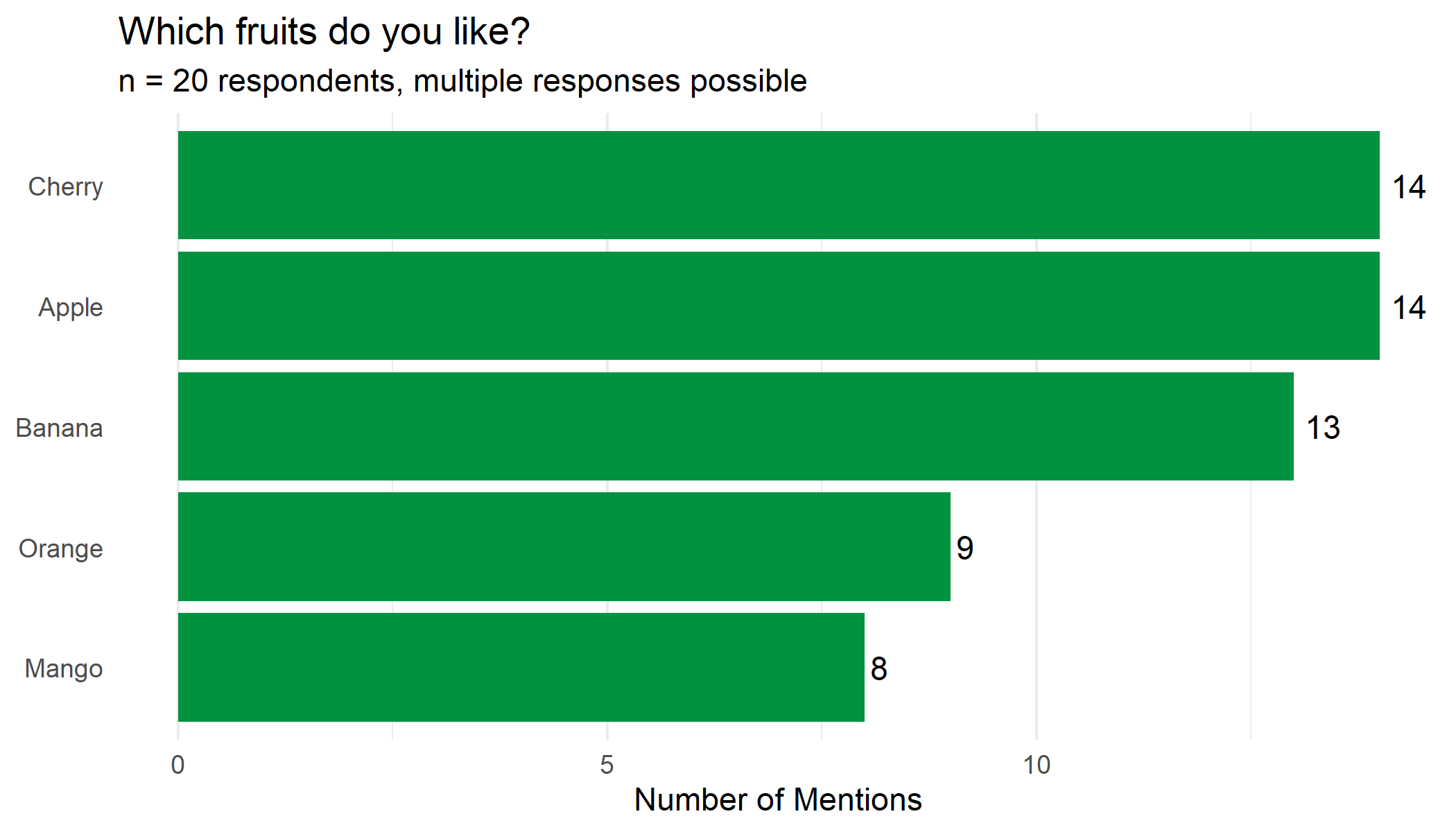
Analysis: Cross-Tabulations
Often you want to know whether responses differ between groups. With our grouping variable gender, we can create cross-tabulations - again with the familiar tools:
survey_long %>%
  tabyl(fruit, gender) %>%
  adorn_totals("col") %>%
  adorn_percentages("col") %>%
  adorn_pct_formatting() %>%
  adorn_ns()
fruit f m Total
apple 24.3% (9) 23.8% (5) 24.1% (14)
banana 27.0% (10) 14.3% (3) 22.4% (13)
cherry 24.3% (9) 23.8% (5) 24.1% (14)
mango 16.2% (6) 9.5% (2) 13.8% (8)
orange 8.1% (3) 28.6% (6) 15.5% (9)This table shows for each gender what proportion the respective fruit makes up of all responses in that group. Note: Here too, these are “percent of responses”, not “percent of cases”.
Combination Patterns (Advanced)
Another interesting question: Which fruits are frequently selected together? This analysis goes beyond simple frequencies and examines the patterns in the responses.
The Most Common Combinations
For this, we use the same approach as for format conversion - we pivot to long format and combine the selected options per person:
survey %>%
  pivot_longer(
    cols = starts_with("Q1_"),
    names_to = "fruit",
    names_prefix = "Q1_",
    values_to = "selected"
  ) %>%
  filter(selected == 1) %>%
  summarise(
    combination = str_c(str_to_title(fruit), collapse = " + "),
    .by = person_id
  ) %>%
  count(combination, sort = TRUE, name = "count")
# A tibble: 10 × 2
combination count
<chr> <int>
1 Apple + Banana + Cherry 3
2 Apple + Cherry + Orange 3
3 Banana + Cherry 3
4 Apple + Banana + Orange 2
5 Apple + Cherry + Mango 2
6 Apple + Mango + Orange 2
7 Banana + Cherry + Mango 2
8 Apple + Banana + Cherry + Mango + Orange 1
9 Apple + Banana + Mango 1
10 Banana + Orange 1Overview with UpSet Plot
For visualizing combinations, UpSet plots are better suited than classic Venn diagrams, especially when there are more than three categories. The ggupset package provides a ggplot2 integration:
survey_long %>%
  summarise(
    fruit = list(str_to_title(fruit)),
    .by = person_id
  ) %>%
  ggplot(aes(x = fruit)) +
  geom_bar(fill = "#00923f") +
  scale_x_upset() +
  labs(
    x = NULL,
    y = "Number of Persons",
    title = "Combination Patterns of Fruit Preferences"
  ) +
  theme_minimal()
Warning: Using `size` aesthetic for lines was deprecated in ggplot2 3.4.0.
ℹ Please use `linewidth` instead.
ℹ The deprecated feature was likely used in the ggupset package.
Please report the issue at <https://github.com/const-ae/ggupset/issues>.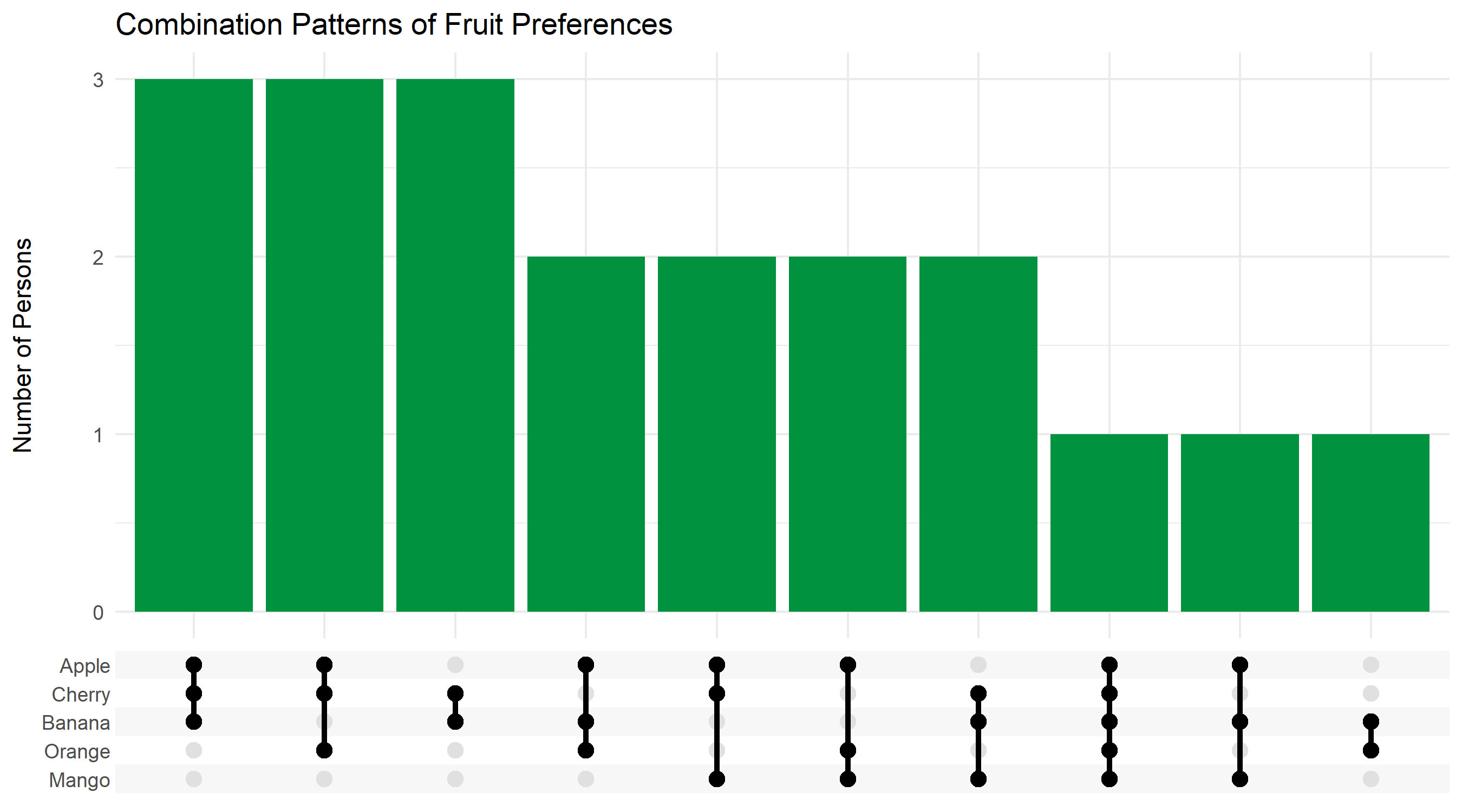
TipExercise: Your Own Analysis
Analyze the survey dataset further:
- Calculate the average number of selected fruits per person.
- Is there a difference between men and women in the number of selected options?
- Which fruit is most frequently selected as the only option (i.e., by people who like only one fruit)?
NoteSolution
1. Average number per person
# A tibble: 1 × 4
   mean median   min   max
  <dbl>  <dbl> <dbl> <dbl>
1   2.9      3     2     5
2. Difference by gender
# A tibble: 2 × 2
  gender  mean
  <chr>  <dbl>
1 m       2.62
2 f       3.08
3. Most common single choice
# A tibble: 0 × 2
# ℹ 2 variables: fruit <chr>, n <int>
Summary
Multiple responses require special attention to data structure and analysis:
- Three common formats: Dichotomous (0/1 columns), Collapsed (delimited), Long (one row per response)
-
Column prefixes: Related columns often share a common prefix (e.g.,
Q1_) that can be selected withstarts_with() -
Conversion: With
pivot_longer(),pivot_wider(),separate_longer_delim(), andsummarise(), all formats can be converted to each other -
Frequency tables: In long format,
tabyl()works as usual - Two percentage types: Percent of cases (base: persons) vs. percent of responses (base: all responses)
- Cross-tabulations: Grouping variables enable comparisons between subgroups
- Combination patterns: Show which options are frequently selected together (UpSet plot)
Citation
BibTeX citation:
@online{schmidt2026,
  author = {{Dr. Paul Schmidt}},
  publisher = {BioMath GmbH},
  title = {6. {Analyzing} {Multiple} {Response} {Questions}},
  date = {2026-06-08},
  url = {https://biomathcontent.netlify.app/content/r_more/06_multiple_response.html},
  langid = {en}
}
For attribution, please cite this work as:
Dr. Paul Schmidt. 2026. “6. Analyzing Multiple Response
Questions.” BioMath GmbH. June 8, 2026. https://biomathcontent.netlify.app/content/r_more/06_multiple_response.html.