---
title: "8. Writing Functions"
subtitle: "Creating reusable code and understanding tidy evaluation"
---
```{r}
#| label: func-setup
#| include: false
# Packages
for (pkg in c("tidyverse", "rlang")) {
if (!require(pkg, character.only = TRUE)) install.packages(pkg)
}
library(tidyverse)
library(rlang)
```
## Why Write Functions?
One of the most important steps on the journey from R user to R programmer is writing your own functions. The basic principle is simple: if you've copied and pasted the same code more than twice, you should turn it into a function. This rule is often called the **DRY principle** — "Don't Repeat Yourself".
Writing functions has several tangible benefits. First, you can give your function a meaningful name that immediately reveals what the code does. Second, when changes are needed, you only have to modify one place in the code, not every copy. Third, you eliminate errors that arise from copying and pasting — like forgetting to change a variable name in one place. And fourth, you can reuse your functions across projects.
Consider the following code that scales columns to a range of 0 to 1:
```{r}
#| label: func-motivation-problem
mtcars %>%
  select(mpg, hp, wt, qsec) %>%
  mutate(
    mpg = (mpg - min(mpg, na.rm = TRUE)) / (max(mpg, na.rm = TRUE) - min(mpg, na.rm = TRUE)),
    hp = (hp - min(hp, na.rm = TRUE)) / (max(hp, na.rm = TRUE) - min(hp, na.rm = TRUE)),
    wt = (wt - min(wt, na.rm = TRUE)) / (max(hp, na.rm = TRUE) - min(wt, na.rm = TRUE)),
    qsec = (qsec - min(qsec, na.rm = TRUE)) / (max(qsec, na.rm = TRUE) - min(qsec, na.rm = TRUE))
  ) %>%
  head()
```
This code is not only long and repetitive, it also contains a subtle bug — can you spot it? With so much repetition, it's almost inevitable that typos creep in. A function solves both problems.
:::{.callout-tip}
## Further Resources
This chapter is strongly based on the excellent [Chapter 25: Functions](https://r4ds.hadley.nz/functions.html) from "R for Data Science" (2nd edition). For a deeper treatment of tidy evaluation, we recommend the [Programming with dplyr](https://dplyr.tidyverse.org/articles/programming.html) vignette.
:::
## Basics: function()
### Syntax and Structure
A function in R consists of three parts: a **name**, the **arguments**, and the **body**. The basic syntax looks like this:
```{r}
#| label: func-basic-syntax
#| eval: false
function_name <- function(argument1, argument2) {
  # Body: The code that gets executed
  result <- argument1 + argument2
  result
}
```
Let's apply this to our scaling problem. The repeating part is the formula `(x - min(x)) / (max(x) - min(x))`. The only thing that changes is the variable — that becomes our argument:
```{r}
#| label: func-rescale01
rescale01 <- function(x) {
  rng <- range(x, na.rm = TRUE)
  (x - rng[1]) / (rng[2] - rng[1])
}
```
Let's test the function:
```{r}
#| label: func-rescale01-test
rescale01(c(-10, 0, 10))
rescale01(c(1, 2, 3, NA, 5))
```
Now our original code becomes much more readable and shorter:
```{r}
#| label: func-rescale01-usage
mtcars %>%
  select(mpg, hp, wt, qsec) %>%
  mutate(
    mpg = rescale01(mpg),
    hp = rescale01(hp),
    wt = rescale01(wt),
    qsec = rescale01(qsec)
  ) %>%
  head()
```
### Arguments With and Without Defaults
Functions can have any number of arguments. Arguments without a default value are **required**, arguments with a default value are **optional**:
```{r}
#| label: func-arguments-demo
# na.rm has a default value, x does not
my_mean <- function(x, na.rm = FALSE) {
  sum(x, na.rm = na.rm) / length(x)
}

my_mean(c(1, 2, 3))
my_mean(c(1, 2, NA), na.rm = TRUE)
```
For ordering: required arguments come first, optional ones after. The most important argument (usually the data) comes first — this enables seamless integration into pipe chains.
### Return Values
R functions automatically return the result of the last line. You can also explicitly use `return()`, which is especially useful for early exits:
```{r}
#| label: func-return-demo
# Implicit return (last line)
add_one <- function(x) {
  x + 1
}

# Explicit return with return()
safe_divide <- function(x, y) {
  if (y == 0) {
    return(NA_real_)
  }
  x / y
}

safe_divide(10, 2)
safe_divide(10, 0)
```
The convention is: use `return()` only for early exits. At the end of the function, implicit return is more common and readable.
### The Ellipsis Argument (...)
The special argument `...` (three dots, also called "ellipsis") allows passing any number of additional arguments through to another function:
```{r}
#| label: func-ellipsis-demo
# All additional arguments are passed to mean()
my_summary <- function(x, ...) {
  c(
    mean = mean(x, ...),
    sd = sd(x, ...)
  )
}

# Without na.rm
my_summary(c(1, 2, 3))
# With na.rm = TRUE (passed through to mean() and sd())
my_summary(c(1, 2, NA), na.rm = TRUE)
```
This is especially useful when writing wrapper functions and you don't want to explicitly list all possible arguments of the inner function.
:::{.callout-tip collapse="false"}
## Exercise: Coefficient of Variation
Write a function `cv()` that calculates the coefficient of variation (standard deviation divided by mean). The function should have an optional `na.rm` argument.
```{r}
#| label: func-exercise-cv-task
#| eval: false
cv(c(1, 2, 3, 4, 5))
cv(c(1, 2, NA, 4, 5), na.rm = TRUE)
```
:::
:::{.callout-note collapse="true"}
## Solution
```{r}
#| label: func-exercise-cv-solution
cv <- function(x, na.rm = FALSE) {
  sd(x, na.rm = na.rm) / mean(x, na.rm = na.rm)
}

cv(c(1, 2, 3, 4, 5))
cv(c(1, 2, NA, 4, 5), na.rm = TRUE)
```
:::
## Three Types of Functions
The R for Data Science book distinguishes three useful categories of functions that you'll frequently write.
### Vector Functions
Vector functions take one or more vectors as input and return a vector. They can be further divided into **mutate functions** (output has the same length as input) and **summary functions** (output has length 1).
```{r}
#| label: func-vector-types
# Mutate function: same length as input
z_score <- function(x) {
  (x - mean(x, na.rm = TRUE)) / sd(x, na.rm = TRUE)
}

z_score(c(1, 2, 3, 4, 5))
# Summary function: single value as output
coef_variation <- function(x, na.rm = FALSE) {
  sd(x, na.rm = na.rm) / mean(x, na.rm = na.rm)
}

coef_variation(c(1, 2, 3, 4, 5))
```
### Dataframe Functions
Dataframe functions take a dataframe as input and return a dataframe. They are typically wrappers around dplyr verbs:
```{r}
#| label: func-dataframe-type
# Example of a dataframe function
filter_extreme <- function(df, var, threshold = 2) {
  df %>%
    filter(abs(as.vector(scale({{ var }}))) > threshold)
}

# Cars with extreme fuel consumption (> 2 SD from mean)
mtcars %>%
  filter_extreme(mpg) %>%
  select(mpg, hp, wt)
```
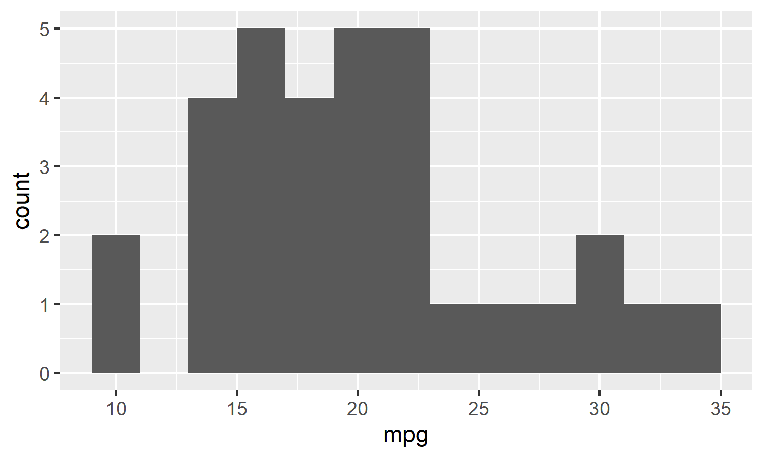
### Plot Functions
Plot functions take a dataframe and return a ggplot:
```{r}
#| label: func-plot-type
#| fig-width: 5
#| fig-height: 3
# Example of a plot function
histogram <- function(df, var, binwidth = NULL) {
  df %>%
    ggplot(aes(x = {{ var }})) +
    geom_histogram(binwidth = binwidth)
}

mtcars %>% histogram(mpg, binwidth = 2)
```
The `{ }` syntax in the plot example will be explained in detail in the section on tidy evaluation.
## Defensive Programming
Good functions check their inputs and provide understandable error messages. This saves debugging time and makes the code more robust.
### stop() for Error Messages
The `stop()` function aborts execution and displays an error message:
```{r}
#| label: func-stop-demo
#| error: true
calculate_bmi <- function(weight_kg, height_m) {
  if (!is.numeric(weight_kg) || !is.numeric(height_m)) {
    stop("weight_kg and height_m must be numeric")
  }
  if (any(height_m <= 0)) {
    stop("height_m must be positive")
  }
  weight_kg / height_m^2
}

calculate_bmi(70, 1.75)
calculate_bmi(70, "tall")
```
### stopifnot() for Quick Checks
For simple conditions, `stopifnot()` is more compact:
```{r}
#| label: func-stopifnot-demo
#| error: true
calculate_bmi <- function(weight_kg, height_m) {
  stopifnot(is.numeric(weight_kg), is.numeric(height_m))
  stopifnot(all(height_m > 0))

  weight_kg / height_m^2
}

calculate_bmi(70, 0)
```
The downside: the automatically generated error messages are less informative than custom ones.
### match.arg() for Categorical Arguments
When an argument should only accept certain values, use `match.arg()`:
```{r}
#| label: func-matcharg-demo
#| error: true
center <- function(x, type = c("mean", "median", "trimmed")) {
  type <- match.arg(type)

  switch(type,
    mean = mean(x, na.rm = TRUE),
    median = median(x, na.rm = TRUE),
    trimmed = mean(x, trim = 0.1, na.rm = TRUE)
  )
}

center(1:10, "mean")
center(1:10, "median")
center(1:10, "mena")
```
The allowed values are defined in the argument's default. `match.arg()` also allows partial matching and provides helpful error messages for invalid inputs.
:::{.callout-tip collapse="false"}
## Exercise: Safe Logarithm Function
Write a function `safe_log()` that:
1. Checks if the input is numeric
2. Checks if all values are positive
3. For non-positive values, gives a helpful error message indicating how many non-positive values are present
```{r}
#| label: func-exercise-safelog-task
#| eval: false
safe_log(c(1, 10, 100))
safe_log(c(-1, 10, 100))
```
:::
:::{.callout-note collapse="true"}
## Solution
```{r}
#| label: func-exercise-safelog-solution
#| error: true
safe_log <- function(x, base = exp(1)) {
  if (!is.numeric(x)) {
    stop("x must be numeric, not ", typeof(x))
  }

  n_negative <- sum(x <= 0, na.rm = TRUE)
  if (n_negative > 0) {
    stop(
      glue::glue("x contains {n_negative} value(s) <= 0. ",
                 "Logarithm is only defined for positive numbers.")
    )
  }

  log(x, base = base)
}

safe_log(c(1, 10, 100))
safe_log(c(-1, 0, 10, 100))
```
:::
## Functions in the tidyverse: Tidy Evaluation
Once you start writing functions that use tidyverse verbs like `filter()`, `mutate()`, or `ggplot()`, you encounter a special problem: how do you pass column names as arguments?
### The Problem: Indirection
Consider this naive function:
```{r}
#| label: func-indirection-problem
#| error: true
grouped_mean <- function(df, group_var, mean_var) {
  df %>%
    group_by(group_var) %>%
    summarize(mean = mean(mean_var))
}

mtcars %>% grouped_mean(cyl, mpg)
```
The function looks for columns named `group_var` and `mean_var` — but they don't exist! The problem is **indirection**: dplyr uses **data masking** to allow column names without quotes. This is convenient for interactive use but makes writing functions more complicated.
:::{.callout-note}
## Data Masking Explained
Data masking means you can write `filter(df, x > 5)` instead of `filter(df, df$x > 5)`. R looks for `x` first in the dataframe's columns, then in the environment. That's why `group_var` is interpreted as a column name — not as a variable containing a column name.
:::
### The Standard Solution: Curly-Curly
Since rlang 0.4.0 (2019) there's an elegant solution: the **embracing operator** `{ }` (also called "curly-curly"). It tells dplyr: "Don't look for a column with this name, look inside this variable instead":
```{r}
#| label: func-curly-curly-solution
grouped_mean <- function(df, group_var, mean_var) {
  df %>%
    group_by({{ group_var }}) %>%
    summarize(mean = mean({{ mean_var }}), .groups = "drop")
}

mtcars %>% grouped_mean(cyl, mpg)
```
The rule is simple: **embrace every argument that is passed to a tidyverse function that uses data masking or tidy selection.**
How do you know which functions use these? The documentation tells you: look for `<data-masking>` (for functions like `filter()`, `mutate()`, `summarize()`) or `<tidy-select>` (for functions like `select()`, `rename()`, `across()`).
```{r}
#| label: func-curly-curly-examples
# Flexible summary function
summary_stats <- function(df, var) {
  df %>%
    summarize(
      n = n(),
      mean = mean({{ var }}, na.rm = TRUE),
      sd = sd({{ var }}, na.rm = TRUE),
      min = min({{ var }}, na.rm = TRUE),
      max = max({{ var }}, na.rm = TRUE)
    )
}

mtcars %>% summary_stats(mpg)
mtcars %>% group_by(cyl) %>% summary_stats(mpg)
```
:::{.callout-tip collapse="false"}
## Exercise: Counting Proportions
Write a function `count_prop()` that works like `count()` but additionally adds a `prop` column with the proportion.
```{r}
#| label: func-exercise-countprop-task
#| eval: false
# Desired result:
mtcars %>% count_prop(cyl)
# # A tibble: 3 × 3
#     cyl     n  prop
#   <dbl> <int> <dbl>
# 1     4    11 0.344
# 2     6     7 0.219
# 3     8    14 0.438
```
:::
:::{.callout-note collapse="true"}
## Solution
```{r}
#| label: func-exercise-countprop-solution
count_prop <- function(df, var, sort = FALSE) {
  df %>%
    count({{ var }}, sort = sort) %>%
    mutate(prop = n / sum(n))
}

mtcars %>% count_prop(cyl)
```
:::
### Dynamic Column Names with the Walrus Operator
What if you want to not just *read* a column, but *create* a column with a dynamic name? The normal `=` operator only allows fixed names on the left side. This is where `:=` comes in (the "walrus operator"):
```{r}
#| label: func-walrus-operator
# Function that creates a new column with dynamic name
standardize <- function(df, var) {
  df %>%
    mutate(
      "{{ var }}_z" := ({{ var }} - mean({{ var }}, na.rm = TRUE)) /
                       sd({{ var }}, na.rm = TRUE)
    )
}

mtcars %>%
  select(mpg, cyl) %>%
  standardize(mpg) %>%
  head()
```
The syntax `"{{ var }}_z" :=` combines glue-style string interpolation with the walrus operator. The `{ var }` in the string is replaced by the variable name.
### Columns as Strings: .data Pronoun
Sometimes you have column names as strings — perhaps from a configuration file or user input. Here you use the `.data` pronoun:
```{r}
#| label: func-data-pronoun
# Column name comes as string
summarize_column <- function(df, col_name) {
  df %>%
    summarize(mean = mean(.data[[col_name]], na.rm = TRUE))
}

summarize_column(mtcars, "mpg")
# Useful for iteration over column names
col_names <- c("mpg", "hp", "wt")
map(col_names, ~ summarize_column(mtcars, .x))
```
### Advanced: enquo() and !!
The `{ }` syntax is shorthand for a combination of `enquo()` and `!!`. In most cases you don't need the explicit form, but there are situations where it's necessary — for example when you want to extract the variable name as a string.
Here's the same function in both notations:
```{r}
#| label: func-enquo-comparison
# With {{ }} - the recommended shorthand
grouped_mean_short <- function(df, group_var, mean_var) {
  df %>%
    group_by({{ group_var }}) %>%
    summarize(mean = mean({{ mean_var }}), .groups = "drop")
}

# With enquo() and !! - the explicit form
grouped_mean_explicit <- function(df, group_var, mean_var) {
  group_var <- enquo(group_var)  # Capture the argument
  mean_var <- enquo(mean_var)

  df %>%
    group_by(!!group_var) %>%    # Insert with !!
    summarize(mean = mean(!!mean_var), .groups = "drop")
}

# Both produce the same result
mtcars %>% grouped_mean_short(cyl, mpg)
mtcars %>% grouped_mean_explicit(cyl, mpg)
```
**enquo()** captures an argument without evaluating it. **!!** (bang-bang) inserts the captured expression.
When do you need the explicit form? When you want to extract the variable name as a string:
```{r}
#| label: func-enquo-aslabel
# as_label() extracts the name as string - only possible with enquo()
summary_with_label <- function(df, var) {
  var_quo <- enquo(var)
  var_name <- rlang::as_label(var_quo)

  df %>%
    summarize(
      variable = var_name,
      mean = mean(!!var_quo, na.rm = TRUE)
    )
}

mtcars %>% summary_with_label(mpg)
mtcars %>% summary_with_label(hp)
```
### Multiple Columns as Strings: syms() and !!!
When you have multiple column names as a character vector and want to use them in a tidyverse function, you need `syms()` and `!!!`:
- **syms()** converts a character vector into a list of symbols
- **!!!** (splice operator) unpacks this list so each element is passed individually
```{r}
#| label: func-splice-demo
# Multiple grouping variables as character vector
grouped_summary <- function(df, group_vars, summary_var) {
  # syms() converts c("cyl", "am") to list(sym("cyl"), sym("am"))
  group_symbols <- syms(group_vars)

  df %>%
    # !!! unpacks the list: group_by(cyl, am) instead of group_by(list(...))
    group_by(!!!group_symbols) %>%
    summarize(mean = mean({{ summary_var }}, na.rm = TRUE), .groups = "drop")
}

mtcars %>% grouped_summary(c("cyl", "am"), mpg)
```
This technique is especially useful when grouping variables are determined dynamically — perhaps from a configuration or user input.
### pick() for Tidy Selection in Data-Masking Context
Sometimes you want to use tidy selection (like in `select()`) inside a data-masking function (like `group_by()`). This is where `pick()` helps:
```{r}
#| label: func-pick-demo
# Multiple grouping columns with tidy selection
count_by <- function(df, ...) {
  df %>%
    group_by(pick(...)) %>%
    summarize(n = n(), .groups = "drop")
}

mtcars %>% count_by(cyl, am)
mtcars %>% count_by(starts_with("c"))
```
Important: with `...` you use `pick(...)` directly, not `pick({{ ... }})`. The `{ }` syntax is only for single named arguments.
### Overview: When to Use Which Approach?
| Situation | Solution | Example |
|-----------|----------|---------|
| Column as "bare name" | `{ }` | `filter({{ var }} > 0)` |
| Column name as string | `.data[[]]` | `summarize(mean = mean(.data[[col]]))` |
| Multiple columns via `...` | Pass `...` directly | `group_by(...)` or `pick(...)` |
| Create dynamic column name | `:=` | `mutate("{{ var }}_new" := ...)` |
| Extract variable name as string | `enquo()` + `as_label()` | `as_label(enquo(var))` |
| List of strings to symbols | `syms()` + `!!!` | `group_by(!!!syms(cols))` |
| Tidy select in data masking | `pick()` | `group_by(pick(...))` |
:::{.callout-tip collapse="false"}
## Exercise: Flexible Filtering
Write a function `filter_na()` that removes all rows where a specific column is `NA`.
```{r}
#| label: func-exercise-filtna-task
#| eval: false
# Test data
test_df <- tibble(
  x = c(1, NA, 3),
  y = c("a", "b", NA)
)

test_df %>% filter_na(x)
test_df %>% filter_na(y)
```
:::
:::{.callout-note collapse="true"}
## Solution
```{r}
#| label: func-exercise-filtna-solution
filter_na <- function(df, var) {
  df %>%
    filter(!is.na({{ var }}))
}

test_df <- tibble(
  x = c(1, NA, 3),
  y = c("a", "b", NA)
)

test_df %>% filter_na(x)
test_df %>% filter_na(y)
```
:::
:::{.callout-tip collapse="false"}
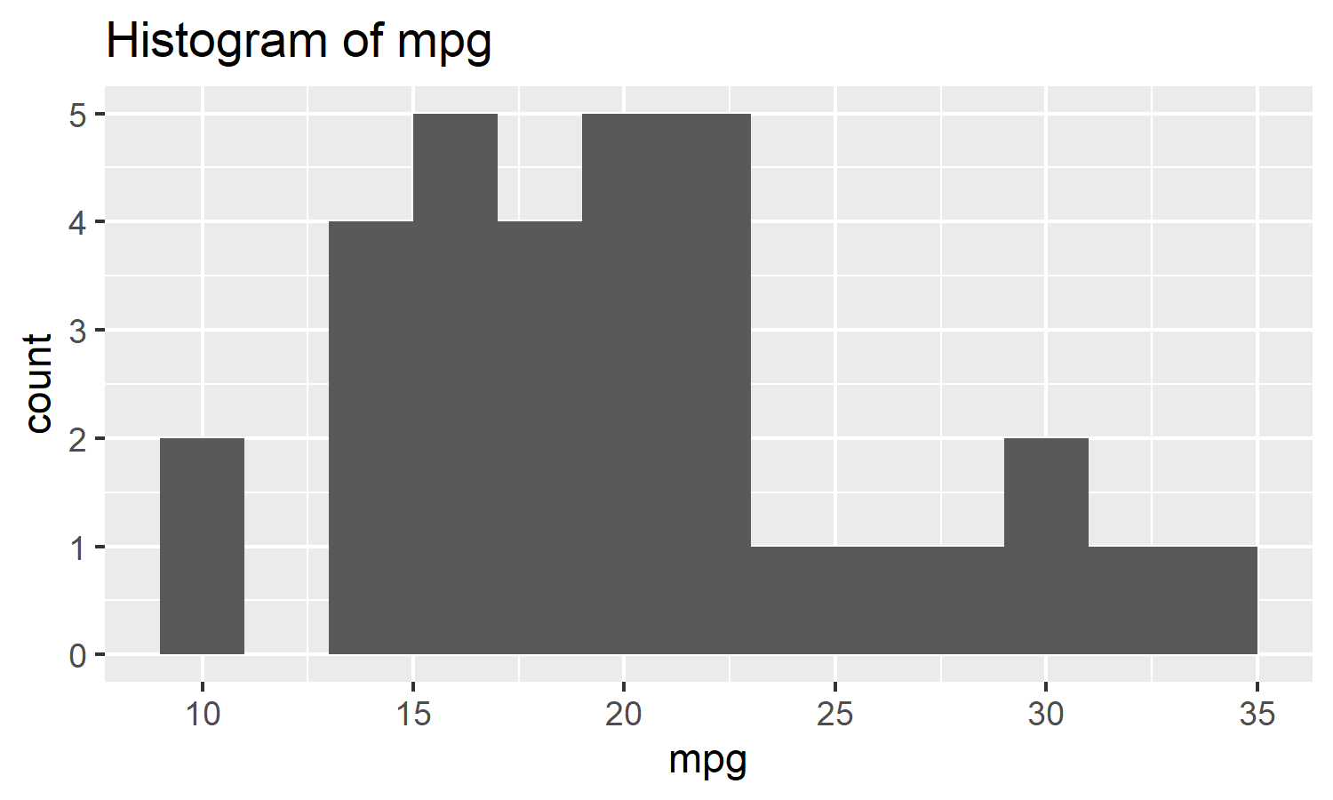
## Exercise: Plot Function with Dynamic Title
Extend the `histogram()` function so that the title automatically includes the variable name:
```{r}
#| label: func-exercise-plottitle-task
#| eval: false
mtcars %>% histogram(mpg, binwidth = 2)
# Should have a title like "Histogram of mpg"
```
*Hint: Use `rlang::englue()` or the combination of `enquo()` and `as_label()`.*
:::
:::{.callout-note collapse="true"}
## Solution
```{r}
#| label: func-exercise-plottitle-solution
#| fig-width: 5
#| fig-height: 3
histogram <- function(df, var, binwidth = NULL) {
  title <- rlang::englue("Histogram of {{var}}")

  df %>%
    ggplot(aes(x = {{ var }})) +
    geom_histogram(binwidth = binwidth) +
    labs(title = title)
}

mtcars %>% histogram(mpg, binwidth = 2)
```
:::
## Best Practices and Style
### Naming
Function names should be verbs and clearly describe what the function does:
```{r}
#| label: func-naming
#| eval: false
# Good: Verbs, descriptive
impute_missing()
calculate_bmi()
extract_coefficients()

# Bad: Too short or not descriptive
f()
my_function()
do_stuff()
```
Argument names should be nouns. The data argument is typically called `df`, `data`, or `.data`.
### Code Formatting
Always use curly braces `{}`, even for single-line functions. The body is indented with two spaces:
```{r}
#| label: func-style
#| eval: false
# Good
add_one <- function(x) {
  x + 1
}

# Avoid
add_one <- function(x) x + 1
```
### Documentation with Roxygen
When developing an R package, every exported function must be documented. This documentation is written in **Roxygen format** — special comments directly above the function that start with `#'`. When building the package, these comments are automatically converted into the formatted help pages that you access with `?functionname`.
But even if you're not writing a package, just a script with a few helper functions, this format is worthwhile. Instead of writing unstructured comments next to the function, you can use the Roxygen format directly. It's clear, standardized, and if the function later moves into a package, the documentation is already done.
The most important Roxygen tags:
- **Title** (first line): A short, one-line description of the function
- **Description** (after blank line): More detailed explanation of what the function does
- **`@param name`**: Describes an argument of the function
- **`@return`**: Describes what the function returns
- **`@examples`**: Executable examples of usage
```{r}
#| label: func-roxygen-demo
#| eval: false
#' Calculate Body Mass Index
#'
#' This function calculates BMI from weight and height.
#' For vectors, BMI is calculated element-wise.
#'
#' @param weight_kg Weight in kilograms (numeric vector).
#' @param height_m Height in meters (numeric vector).
#'
#' @return A numeric vector of BMI values.
#'
#' @examples
#' calculate_bmi(70, 1.75)
#' calculate_bmi(c(60, 80), c(1.60, 1.80))
calculate_bmi <- function(weight_kg, height_m) {
  stopifnot(is.numeric(weight_kg), is.numeric(height_m))
  stopifnot(all(height_m > 0))

  weight_kg / height_m^2
}
```
In RStudio and Positron you can automatically insert an empty Roxygen skeleton: place the cursor in the function and choose **Code → Insert Roxygen Skeleton** (or `Ctrl+Alt+Shift+R`).