for (pkg in c("agridat", "desplot", "emmeans", "ggtext", "here", "lme4",
              "lmerTest", "multcomp", "multcompView", "tidyverse")) {
  if (!require(pkg, character.only = TRUE)) install.packages(pkg)
}

library(agridat)
library(desplot)
library(emmeans)
library(ggtext)
library(here)
library(lme4)
library(lmerTest)
library(multcomp)
library(multcompView)
library(tidyverse)To install and load all the packages used in this chapter, run the following code:
From Complete to Incomplete Blocks
In the previous chapters, we analyzed data from designs where each block contained all treatments: the RCBD had each cultivar appearing once per block, and the Latin Square had each treatment appearing once per row and once per column. These are called complete block designs.
However, when the number of treatments becomes large, it may not be practical or even possible to fit all treatments into a single block. For example, if we have 24 genotypes and our field plots can only accommodate 4 plots per block due to soil heterogeneity constraints, we cannot use a complete block design. This is where incomplete block designs come in.
What is an Alpha Design?
An alpha design (also called α-design) is a type of resolvable incomplete block design. “Resolvable” means that the incomplete blocks can be grouped into complete replicates, where each replicate contains every treatment exactly once. Within each replicate, treatments are distributed across multiple smaller incomplete blocks.
The advantages of alpha designs include:
- Handling many treatments: Practical when complete blocks would be too large
- Local error control: Smaller blocks are more homogeneous, reducing experimental error
- Resolvability: Complete replicates allow for traditional replicate-based analysis as a fallback
- Flexibility: Can accommodate various numbers of treatments and block sizes
Introduction to Mixed Models
In the previous chapters, we used lm() to fit our models, treating all effects as fixed. For incomplete block designs, we typically use mixed models, which contain both fixed effects (like our treatment/genotype effect) and random effects (like incomplete block effects). We use the lmer() function from the {lmerTest} package to fit mixed models, where random effects are specified with (1 | factor) instead of + factor.
TipBackground reading
For the theoretical background on mixed models - why we treat blocks as random, what BLUEs vs. BLUPs are, and how degrees of freedom are approximated - see the appendix chapter Linear Mixed Models.
Data
This example considers data published in John and Williams (1995) from a yield (t/ha) trial laid out as an alpha design. The trial had 24 genotypes (gen), 3 complete replicates (rep) and 6 incomplete blocks (block) within each replicate. The block size was 4, meaning each incomplete block contained 4 of the 24 genotypes.
Import
The data is available as part of the {agridat} package:
dat <- as_tibble(agridat::john.alpha)
dat
# A tibble: 72 × 7
plot rep block gen yield row col
<int> <fct> <fct> <fct> <dbl> <int> <int>
1 1 R1 B1 G11 4.12 1 1
2 2 R1 B1 G04 4.45 2 1
3 3 R1 B1 G05 5.88 3 1
4 4 R1 B1 G22 4.58 4 1
5 5 R1 B2 G21 4.65 5 1
6 6 R1 B2 G10 4.17 6 1
7 7 R1 B2 G20 4.01 7 1
8 8 R1 B2 G02 4.34 8 1
9 9 R1 B3 G23 4.23 9 1
10 10 R1 B3 G14 4.76 10 1
# ℹ 62 more rowsThe dataset contains:
-
rep: Three complete replicates (R1, R2, R3) -
block: Six incomplete blocks within each replicate (B1-B6) -
gen: 24 genotypes (G01-G24) -
yield: Crop yield in tons per hectare -
rowandcol: Field plot coordinates for visualization
Explore
Let’s first examine the summary statistics by genotype:
# A tibble: 24 × 6
   gen   count mean_yield sd_yield min_yield max_yield
   <fct> <int>      <dbl>    <dbl>     <dbl>     <dbl>
 1 G01       3       5.16    0.534      4.65      5.72
 2 G05       3       5.06    0.841      4.20      5.88
 3 G12       3       4.91    0.641      4.17      5.31
 4 G15       3       4.89    0.207      4.68      5.09
 5 G19       3       4.87    0.398      4.56      5.31
 6 G13       3       4.83    0.619      4.25      5.48
 7 G21       3       4.82    0.503      4.41      5.38
 8 G17       3       4.73    0.379      4.32      5.07
 9 G16       3       4.73    0.502      4.39      5.30
10 G06       3       4.71    0.464      4.25      5.18
# ℹ 14 more rows
Each genotype appears exactly 3 times (once per replicate). Genotype G11 has the highest mean yield, while G24 has the lowest.
Now let’s examine the block structure:
# A tibble: 18 × 4
   rep   block count mean_yield
   <fct> <fct> <int>      <dbl>
 1 R1    B1        4       4.75
 2 R1    B2        4       4.29
 3 R1    B3        4       4.36
 4 R1    B4        4       4.33
 5 R1    B5        4       4.79
 6 R1    B6        4       4.58
 7 R2    B1        4       4.12
 8 R2    B2        4       4.23
 9 R2    B3        4       5.22
10 R2    B4        4       5.01
11 R2    B5        4       5.21
12 R2    B6        4       5.11
13 R3    B1        4       4.38
14 R3    B2        4       3.96
15 R3    B3        4       4.30
16 R3    B4        4       4.22
17 R3    B5        4       4.15
18 R3    B6        4       3.61
We can see that each of the 18 incomplete blocks (6 blocks × 3 replicates) contains exactly 4 plots. Let’s visualize the data:
# sort genotypes by mean yield
gen_order <- dat %>%
  group_by(gen) %>%
  summarise(mean = mean(yield)) %>%
  arrange(mean) %>%
  pull(gen) %>%
  as.character()

ggplot(data = dat) +
  aes(
    y = yield,
    x = gen,
    shape = rep
  ) +
  geom_line(
    aes(group = gen),
    color = "darkgrey"
  ) +
  geom_point() +
  scale_x_discrete(
    name = "Genotype",
    limits = gen_order
  ) +
  scale_y_continuous(
    name = "Yield",
    limits = c(0, NA),
    expand = expansion(mult = c(0, 0.05))
  ) +
  scale_shape_discrete(
    name = "Replicate"
  ) +
  guides(shape = guide_legend(nrow = 1)) +
  theme_classic() +
  theme(
    legend.position = "top",
    axis.text.x = element_text(angle = 90, vjust = 0.5)
  )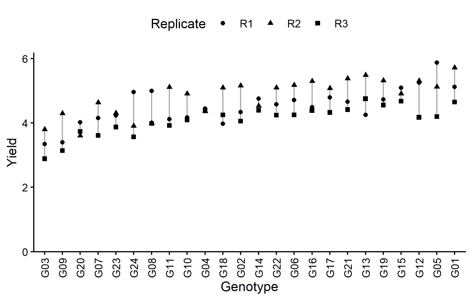
The grey lines connect observations of the same genotype across replicates, helping to visualize genotype consistency. Now let’s look at the field layout:
desplot(
  data = dat,
  flip = TRUE,
  form = gen ~ col + row | rep, # fill color per genotype, panels per replicate
  out1 = block, # lines between incomplete blocks
  out1.gpar = list(col = "black", lwd = 1, lty = "dashed"),
  main = "Field layout",
  key.cex = 0.6,
  layout = c(3, 1) # force all reps in one row
)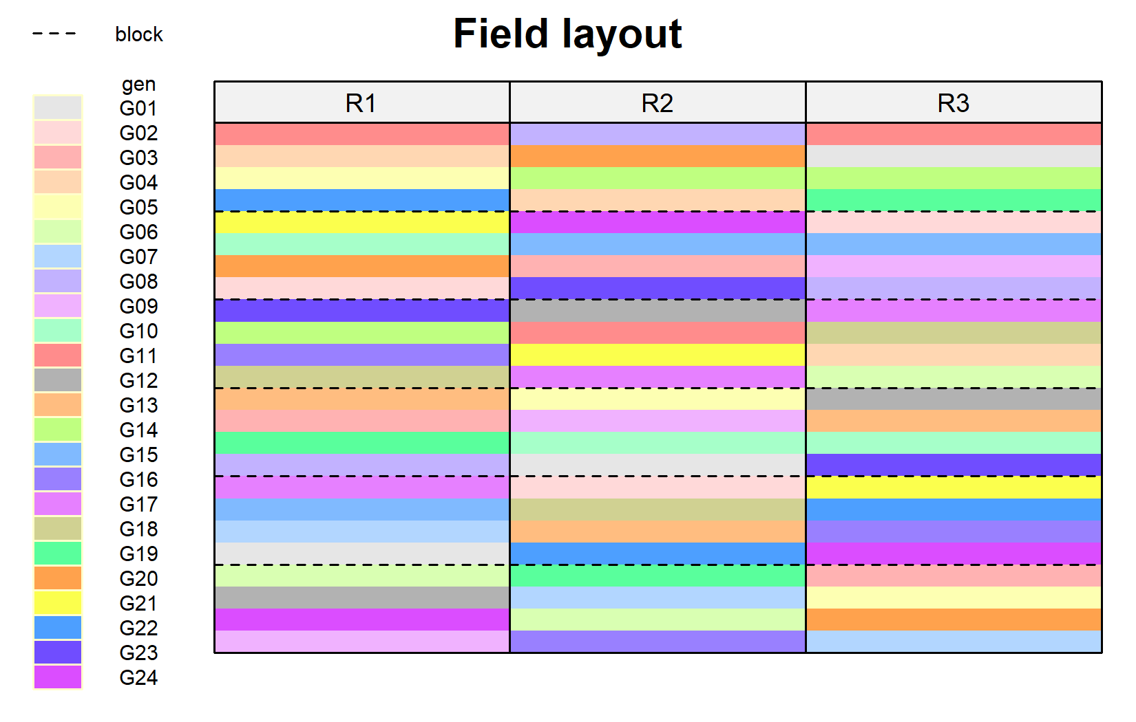
The dashed lines separate the incomplete blocks within each replicate. Notice how each genotype appears once per replicate, but in different blocks.
Model and ANOVA
Model with Random Incomplete Blocks
For an alpha design, the model includes:
- Fixed effects: genotype (
gen) and replicate (rep) - Random effects: incomplete blocks nested within replicates (
rep:block)
The incomplete blocks are treated as random because we are not interested in the specific block effects themselves, but rather want to account for the variation they introduce. This is the key difference from our previous analyses.
mod <- lmer(yield ~ gen + rep + (1 | rep:block),
            data = dat)
The syntax (1 | rep:block) specifies that the interaction of rep and block (i.e., the 18 unique incomplete blocks) should be treated as a random effect.
WarningModel assumptions met?
It is at this point (i.e. after fitting the model and before interpreting the ANOVA) that one should check whether the model assumptions are met. Find out more in Appendix A1: Model Diagnostics.
Conducting the ANOVA
For mixed models, we use a slightly different ANOVA approach with Kenward-Roger degrees of freedom, which provides more accurate F-tests for small sample sizes:
ANOVA <- anova(mod, ddf = "Kenward-Roger")
ANOVA
Type III Analysis of Variance Table with Kenward-Roger's method
Sum Sq Mean Sq NumDF DenDF F value Pr(>F)
gen 10.5070 0.45683 23 35.498 5.3628 4.496e-06 ***
rep 1.5703 0.78513 2 11.519 9.2124 0.004078 **
---
Signif. codes: 0 '***' 0.001 '**' 0.01 '*' 0.05 '.' 0.1 ' ' 1The ANOVA shows that the genotype effect is statistically significant (p < 0.05), indicating that at least one genotype differs from the others in yield.
Mean Comparisons
As in previous chapters, we use emmeans() to obtain adjusted means and perform post-hoc comparisons:
 gen emmean    SE   df lower.CL upper.CL .group
 G03   3.50 0.199 44.3     3.10     3.90  a
 G09   3.50 0.199 44.3     3.10     3.90  ab
 G20   4.04 0.199 44.3     3.64     4.44   bc
 G07   4.11 0.199 44.3     3.71     4.51    cd
 G24   4.15 0.199 44.3     3.75     4.55    cd
 G23   4.25 0.199 44.3     3.85     4.65    cde
 G11   4.28 0.199 44.3     3.88     4.68    cde
 G18   4.36 0.199 44.3     3.96     4.76    cdef
 G10   4.37 0.199 44.3     3.97     4.77    cdef
 G02   4.48 0.199 44.3     4.08     4.88    cdefg
 G04   4.49 0.199 44.3     4.09     4.89    cdefg
 G22   4.53 0.199 44.3     4.13     4.93    cdefgh
 G08   4.53 0.199 44.3     4.13     4.93    cdefgh
 G06   4.54 0.199 44.3     4.14     4.94    cdefgh
 G17   4.60 0.199 44.3     4.20     5.00     defghi
 G16   4.73 0.199 44.3     4.33     5.13      efghi
 G12   4.76 0.199 44.3     4.35     5.16      efghi
 G13   4.76 0.199 44.3     4.36     5.16      efghi
 G14   4.78 0.199 44.3     4.37     5.18      efghi
 G21   4.80 0.199 44.3     4.39     5.20      efghi
 G19   4.84 0.199 44.3     4.44     5.24       fghi
 G15   4.97 0.199 44.3     4.57     5.37        ghi
 G05   5.04 0.199 44.3     4.64     5.44         hi
 G01   5.11 0.199 44.3     4.71     5.51          i

Results are averaged over the levels of: rep
Degrees-of-freedom method: kenward-roger
Confidence level used: 0.95
significance level used: alpha = 0.05
NOTE: If two or more means share the same grouping symbol,
      then we cannot show them to be different.
      But we also did not show them to be the same.
Note that these means are adjusted for both replicate and incomplete block effects. The compact letter display shows which genotypes are significantly different from each other according to Fisher’s LSD test.
Visualizing Results
my_caption <- "Black dots represent raw data. Red diamonds and error bars represent adjusted means with 95% confidence limits per genotype. Means followed by a common letter are not significantly different according to Fisher's LSD test."

ggplot() +
  aes(x = gen) +
  # black dots representing the raw data
  geom_point(
    data = dat,
    aes(y = yield)
  ) +
  # red diamonds representing the adjusted means
  geom_point(
    data = mean_comp,
    aes(y = emmean),
    shape = 18,
    color = "red",
    position = position_nudge(x = 0.2)
  ) +
  # red error bars representing the confidence limits of the adjusted means
  geom_errorbar(
    data = mean_comp,
    aes(ymin = lower.CL, ymax = upper.CL),
    color = "red",
    width = 0.1,
    position = position_nudge(x = 0.2)
  ) +
  # red letters
  geom_text(
    data = mean_comp,
    aes(y = lower.CL, label = str_trim(.group)),
    color = "red",
    angle = 90,
    hjust = 1.1,
    position = position_nudge(x = 0.2)
  ) +
  scale_x_discrete(
    name = "Genotype",
    limits = as.character(mean_comp$gen)
  ) +
  scale_y_continuous(
    name = "Yield",
    limits = c(0, NA),
    expand = expansion(mult = c(0, 0.05))
  ) +
  labs(caption = my_caption) +
  theme_classic() +
  theme(plot.caption = element_textbox_simple(margin = margin(t = 5)),
        plot.caption.position = "plot",
        axis.text.x = element_text(angle = 90, vjust = 0.5))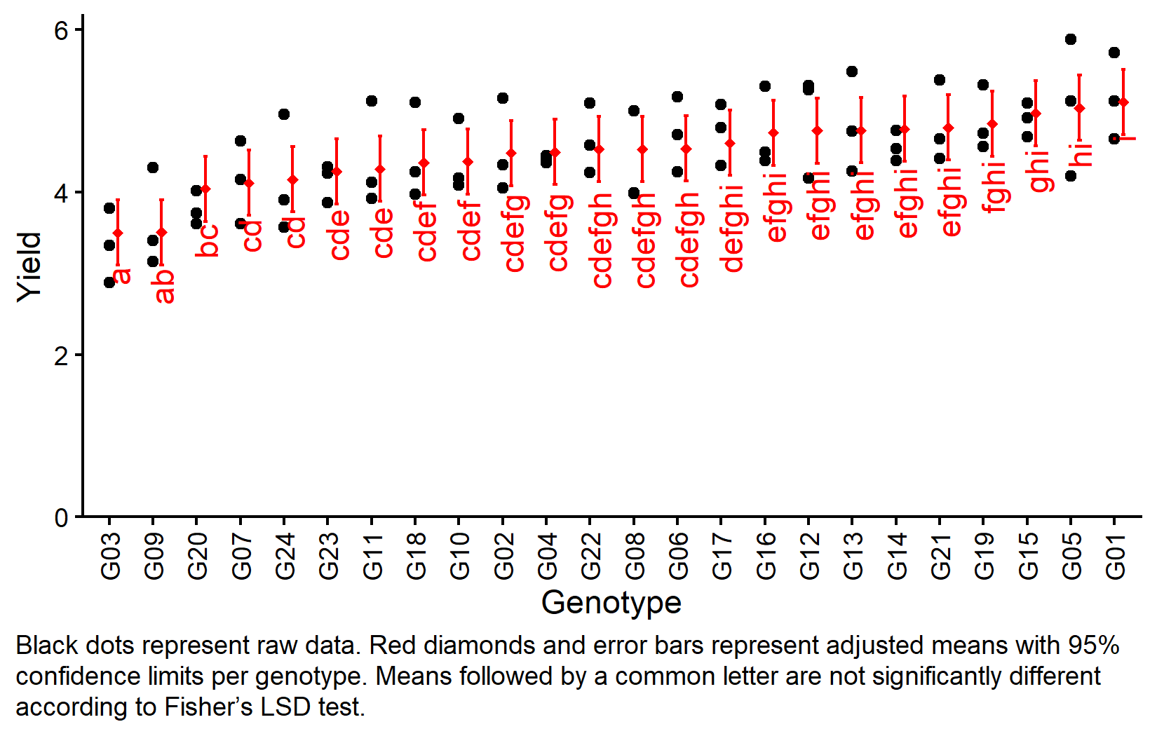
Bonus: Design Efficiency
The efficiency of an incomplete block design can be assessed by comparing it to the analogous RCBD (ignoring incomplete blocks). We compare the squared standard errors of differences:
# s.e.d. squared for alpha design
avg_sed_alpha <- mod %>%
  emmeans(pairwise ~ "gen", adjust = "none", lmer.df = "kenward-roger") %>%
  pluck("contrasts") %>%
  as_tibble() %>%
  pull("SE") %>%
  mean()

# s.e.d. squared for RCBD (ignoring incomplete blocks)
avg_sed_rcbd <- lm(yield ~ gen + rep, data = dat) %>%
  emmeans(pairwise ~ "gen", adjust = "none") %>%
  pluck("contrasts") %>%
  as_tibble() %>%
  pull("SE") %>%
  mean()

# Efficiency
avg_sed_rcbd^2 / avg_sed_alpha^2
[1] 1.230428An efficiency > 1 indicates that the alpha design is more efficient than a simple RCBD, meaning the incomplete blocks successfully reduced experimental error.
Wrapping Up
You’ve now learned how to analyze data from an alpha design, which extends the blocking principle to situations where complete blocks are impractical.
NoteKey Takeaways
Alpha designs are resolvable incomplete block designs useful when the number of treatments is too large for complete blocks.
Mixed models with
lmer()are used to analyze incomplete block designs, treating incomplete blocks as random effects.Random effects syntax: Use
(1 | factor)for random effects instead of+ factorfor fixed effects.The model includes fixed genotype and replicate effects, plus random incomplete block effects:
yield ~ gen + rep + (1 | rep:block).Kenward-Roger degrees of freedom provide more accurate F-tests for mixed models with small sample sizes.
Design efficiency can be assessed by comparing to an analogous RCBD - efficiency > 1 confirms the benefit of incomplete blocking.
References
John, J. A., and E. R. Williams. 1995. “Cyclic and Computer Generated Designs.” Biometrical Journal 38 (7): 778–78. https://doi.org/10.1002/bimj.4710380703.
Citation
BibTeX citation:
@online{schmidt2026,
  author = {{Dr. Paul Schmidt}},
  publisher = {BioMath GmbH},
  title = {4. {One-way} {ANOVA} in an {Alpha} {Design}},
  date = {2026-06-08},
  url = {https://biomathcontent.netlify.app/content/lin_mod_exp/04_oneway_alpha.html},
  langid = {en}
}
For attribution, please cite this work as:
Dr. Paul Schmidt. 2026. “4. One-Way ANOVA in an Alpha
Design.” BioMath GmbH. June 8, 2026. https://biomathcontent.netlify.app/content/lin_mod_exp/04_oneway_alpha.html.