To install and load all the packages used in this chapter, run the following code:
A question that comes up repeatedly in consulting and teaching sounds roughly like this:
I computed adjusted means from my linear model and noticed that the standard errors are all identical across groups. Is that a bug?
It is not a bug. It is a direct consequence of what a standard linear model assumes about the data. This chapter explains where the identical standard errors come from, why they differ from the group-wise standard errors one obtains from descriptive statistics, and how to move to a model that estimates a separate variance per group when that is what the data call for.
Throughout this chapter the term adjusted means is used as shorthand for means that are estimated from a fitted linear model rather than computed directly from the raw observations. Depending on the software or textbook, these are also called:
-
estimated marginal means (the name used by the
{emmeans}package), -
least-squares means (historically
lsmeansin SAS and older R packages), - model-based means or simply predicted means.
All of these refer to the same concept: a mean computed from the model’s coefficients, which therefore inherits the model’s assumptions - including the assumption of a common error variance.
The Quick Version
A default linear model assumes a single, common error variance for all observations (homoscedasticity). Adjusted means are derived from the model’s coefficients, so their standard errors are built from that one variance estimate. With a balanced design this produces exactly the same standard error for every group mean. Group-wise descriptive standard errors differ because they use a separate variance per group.
If the identical standard errors feel wrong, the question to ask is not “why are they the same?” but rather “does my data justify assuming a common variance?” - and that is a question for model diagnostics (see Appendix A1).
A concrete example
Using the built-in PlantGrowth data, a one-way linear model and emmeans() give one standard error per group mean:
 group emmean    SE df lower.CL upper.CL
 ctrl    5.03 0.197 27     4.63     5.44
 trt1    4.66 0.197 27     4.26     5.07
 trt2    5.53 0.197 27     5.12     5.93

Confidence level used: 0.95
Every value in the SE column is 0.197. Now compare this to the same summary computed directly from the data, group by group:
# A tibble: 3 × 5
  group  mean stddev     n stderr
  <fct> <dbl>  <dbl> <int>  <dbl>
1 ctrl   5.03  0.583    10  0.184
2 trt1   4.66  0.794    10  0.251
3 trt2   5.53  0.443    10  0.140
Here the standard errors are clearly different between groups. Both tables describe the same data, so why do they disagree?
Why the descriptive standard errors differ
When a mean, standard deviation, and standard error are computed separately per group, each group is effectively treated as its own sample. Each sample has its own variance estimate, and the standard error of the sample mean follows the textbook formula
\[ \text{SE} = \frac{s}{\sqrt{n}}, \]
where \(s\) is the group’s standard deviation and \(n\) its size. Different groups produce different \(s\), so the standard errors differ.
Why the model-based standard errors are identical
A default linear model assumes that the error variance is the same for every observation, regardless of group. Fitting lm() gives a single pooled variance estimate \(\hat{\sigma}^2\), computed from the residuals across all groups. Every adjusted group mean is then a function of the fitted coefficients, and its standard error is built from that same \(\hat{\sigma}^2\):
\[ \text{SE}(\bar{y}_g) = \sqrt{\hat{\sigma}^2 / n_g}. \]
In a balanced design, where \(n_g\) is the same for every group, the result is one identical standard error for all adjusted means. This is not a quirk of emmeans() - it is the direct mathematical consequence of the homoscedasticity assumption baked into lm(). The underlying assumption is discussed in more depth in Appendix A1 - Model Diagnostics.
- Descriptive means use a separate variance per group, so their standard errors differ.
-
Adjusted means from
lm()share a single pooled variance estimate, so their standard errors are identical (in balanced designs).
Whether you want different or identical standard errors depends on whether a common variance is a reasonable assumption for your data.
Which approach is better?
There is no universal answer: the two approaches rest on different assumptions, and the right choice depends on whether those assumptions match the data. A more useful question is whether the homoscedasticity assumption of the default model is defensible. If it is not, a linear model that allows heterogeneous variances per group is the natural alternative.
Allowing one variance per group
The gls() function from {nlme} fits a generalised least squares model, which accepts a user-specified variance structure via the weights argument. Using varIdent(form = ~ 1 | group) tells the model to estimate a separate residual variance for each level of group:
 group emmean    SE   df lower.CL upper.CL
 ctrl    5.03 0.184 9.01     4.61     5.45
 trt1    4.66 0.251 9.00     4.09     5.23
 trt2    5.53 0.140 9.00     5.21     5.84

Degrees-of-freedom method: satterthwaite
Confidence level used: 0.95
The adjusted means from mod2 now have three different standard errors - and they match the descriptive values computed above. That is expected: with a separate variance per group, the model-based SE reduces to the group-wise formula \(s_g / \sqrt{n_g}\).
Comparing the two models via AIC
Both models describe the same data but make different assumptions. Because mod2 nests mod1 as a special case (the variances could happen to coincide), one can compare them with an information criterion like AIC. Lower AIC indicates the better trade-off between fit and complexity:
AIC(mod1, mod2)Warning in AIC.default(mod1, mod2): Modelle sind nicht alle mit der gleichen
Datensatzgröße angepasst worden df AIC
mod1 4 61.61904
mod2 6 66.98890For PlantGrowth, the simpler homoscedastic model wins. The extra flexibility of fitting three variances instead of one does not buy enough improvement in fit to justify the additional parameters. A quick look at the raw data makes this plausible:
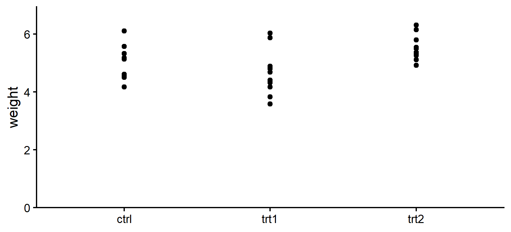
The spread of weight within each group looks broadly comparable. In a scenario where, say, ctrl showed visibly wider scatter than trt1 and trt2, AIC would likely favour the heteroscedastic model.
Beyond the variance question, adjusted means have a practical advantage that group-wise descriptive statistics cannot offer: they come from a model that can include block effects, covariates, or random effects. A descriptive mean for ctrl knows only about the ctrl observations; a model-based mean for ctrl draws information from the full design and adjusts for the other structure in the experiment. For any analysis beyond the simplest one-way layout, model-based means are usually the right target of inference.
Further reading
- Kozak & Piepho (2019): Analyzing designed experiments: Should we report standard deviations or standard errors of the mean or standard errors of the difference or what? - a detailed discussion of which uncertainty measure to report for designed experiments, including the SE vs. SED distinction.
- Stack Exchange: Standard error in estimated marginal means are all the same - with an authoritative answer by Russell Lenth, the author of emmeans.
- Stack Exchange: Interpreting the standard error from emmeans.
- IBM: Estimated Marginal Means all have the same standard error in SPSS - the same phenomenon, seen from the SPSS side.
- Appendix A1 - Model Diagnostics - how to check whether the homoscedasticity assumption behind the identical SEs is reasonable for your data.
Citation
@online{schmidt2026,
  author = {{Dr. Paul Schmidt}},
  title = {A2. {Why} Are the {Standard} {Errors} All the Same?},
  date = {2026-06-08},
  url = {https://biomathcontent.netlify.app/content/lin_mod_exp/a2_whyseequal.html},
  langid = {en}
}