To install and load all the packages used in this chapter, run the following code:
The other chapters in this section walk through the analysis of data that came out of various experimental designs — a CRD in Chapter 1, an RCBD in Chapter 2, a Latin Square in Chapter 3, an alpha design in Chapter 4, an augmented design in Chapter 5, and a resolvable row-column design in Chapter 6. This chapter takes a step back and asks the question that should actually be answered before any data is collected: which design should be used in the first place, and how is it generated?
The Quick Version
Good experimental design is cheaper than good statistics. No amount of modelling can recover information that was never collected, and an unfortunate layout can make even a careful analysis yield ambiguous results. Three principles, all of which go back to Ronald A. Fisher’s classic The Design of Experiments (1935), form the practical core:
- Replication — each treatment must appear more than once, so that the variation between treatments can be separated from the variation within a treatment. Without replication there is no residual variance and therefore no way to judge whether an observed difference is real.
- Randomization — the allocation of treatments to experimental units must be random. Randomization is what justifies the statistical inference in the first place and protects against unknown confounders, such as a gradient in soil fertility or a drift in lab conditions over the course of a day.
- Local control (blocking) — when experimental units are known to differ systematically (e.g. along a slope, between trays, between operators), grouping similar units into blocks and randomizing treatments within each block removes that nuisance variation from the treatment comparison.
If the experimental units are essentially homogeneous and the number of treatments is small, use a CRD. If a single source of heterogeneity can be identified (soil gradient, bench position, day of measurement), use an RCBD. If heterogeneity acts in two orthogonal directions, use a Latin Square (for equal numbers of rows, columns, and treatments) or a resolvable row-column design. If too many treatments exist to fit into a complete block, use an alpha design or another incomplete block design. If many new genotypes need to be screened with limited resources, use an augmented design or a p-rep design.
A strong reference for the practical side of this decision is Casler (2015), which walks through replication, randomization, and blocking with agricultural examples and is worth reading in full before a first field trial.
Choosing a Design
The choice of design is not a matter of taste but a consequence of the experimental question and the experimental material. The following checklist goes through the relevant aspects in the order in which they typically become binding constraints.
Number and type of treatments
The number of treatment levels is usually the first hard constraint. With 3 to 8 treatments, most classical designs remain practical. With 20, 50, or more entries — which is common in plant breeding, where hundreds of candidate genotypes compete for space in a nursery — complete block designs become infeasible and an incomplete block structure is required.
A second consideration is whether the treatments are of equal interest. If all treatments should be estimated with comparable precision, a standard design (CRD, RCBD, alpha) is appropriate. If one group of treatments serves as a reference (checks, standards) and another consists of less-tested entries (new lines, novel formulations), an augmented design (Chapter 5) allocates replications where they matter most.
Structure of the experimental material
Experimental units are rarely truly homogeneous. In a field, fertility tends to vary along a gradient or in patches. In a greenhouse, light and temperature vary with bench position. In a laboratory, batches of reagents or days of measurement introduce variation that has nothing to do with the treatments. Identifying these sources before randomization is what turns a possibly noisy experiment into a clean comparison.
- One direction of heterogeneity — use an RCBD if all treatments fit into a block, or an alpha design if they do not.
- Two orthogonal directions of heterogeneity — use a Latin Square for small, balanced settings or a resolvable row-column design (Chapter 6) for larger trials.
- No identifiable source of heterogeneity — a CRD is the simplest and most efficient choice. Adding blocks “just in case” costs degrees of freedom without a benefit.
Resource constraints
Replication requires experimental units, and units cost money, land, and time. When resources are tight, two strategies are common. Augmented designs keep a small number of replicated checks and add unreplicated test entries alongside, which enables indirect comparisons via the check means. Partially replicated (p-rep) designs replicate only a fraction of the entries (typically 20 to 40 percent), which provides a residual estimate while using substantially fewer plots than full replication. Hans-Peter Piepho et al. (2022) discusses p-rep designs and their trade-offs in detail.
Single-site versus multi-environment trials
Many real experiments are not conducted once but repeated across locations and/or years. The design choice then extends beyond a single site: each location should use an appropriate design for its local conditions, and the set of locations should be chosen so that genotype-by-environment interaction can be estimated. H. P. Piepho, Büchse, and Emrich (2003) and H. P. Piepho, Büchse, and Richter (2004) provide the statistical framework for series of official trials; the practical implication for design generation is that the same script should be run separately per environment, typically with a different random seed, so that spatial patterns are not repeated across sites.
Generating a Design in R
Two R packages cover nearly all designs encountered in practice:
-
{FielDHub} — a modern, well-documented toolbox that also provides a Shiny app. Its functions return a list that includes both the field book (
$fieldBook) and a ready-made ggplot layout ($pinsideplot(out)). -
{agricolae} — the long-standing classic, still useful especially for quick textbook-style designs. Its functions (e.g.
design.crd(),design.rcb(),design.alpha()) return the randomization as a$bookdata frame.
Both are worth knowing. The examples below use FielDHub for layout plots and {agricolae} for a simple text-based randomization.
A CRD with FielDHub
A CRD places treatments on plots without any structural constraints — the randomization is completely free. The following example generates a CRD for four treatments with five replications:
  ID LOCATION PLOT REP TREATMENT
1  1        1  101   3        T3
2  2        1  102   1        T2
3  3        1  103   3        T2
4  4        1  104   5        T1
5  5        1  105   2        T2
6  6        1  106   4        T2
The $fieldBook slot is the actual randomization table — one row per experimental unit, with plot numbers, treatment labels, and any blocking variables. This is the file that is passed on to the field technicians or lab staff who run the experiment.
A simple layout plot can be produced directly with FielDHub:
plot(crd_out)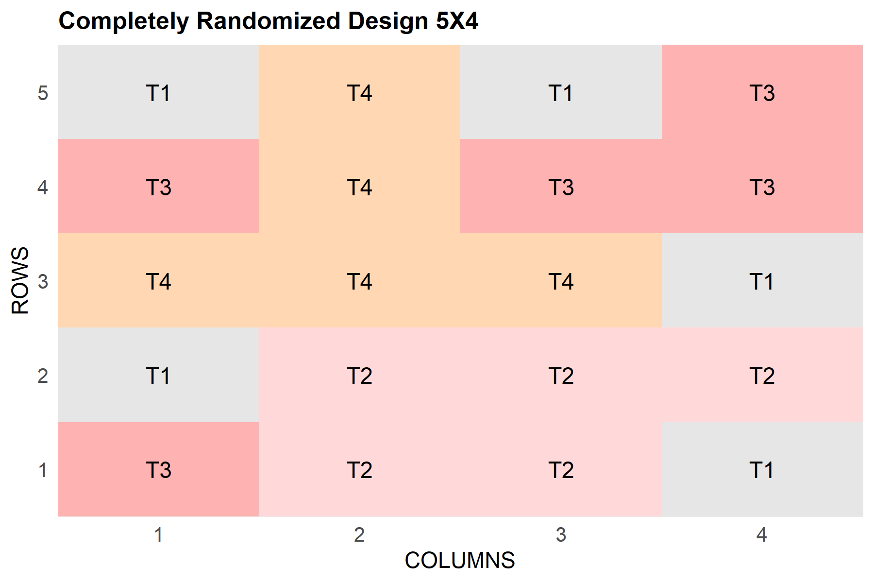
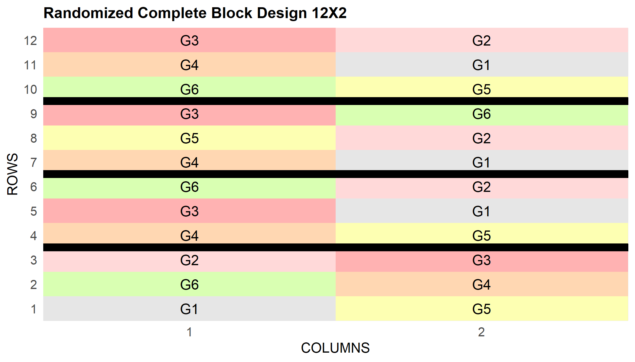
An RCBD and an alpha design
The same pattern works for other designs. For an RCBD with 6 treatments in 4 complete blocks:
And for an alpha design with 15 treatments in incomplete blocks of size 3, replicated 3 times:
alpha_out <- alpha_lattice(
  t    = 15,
  k    = 3,
  r    = 3,
  plotNumber = 101,
  seed = 42
)

plot(alpha_out)
Warning in geom_tileborder(aes(group = 1, grp = .data[[out2.string]]), color =
out2.gpar$col, : Ignoring empty aesthetic: `linewidth`.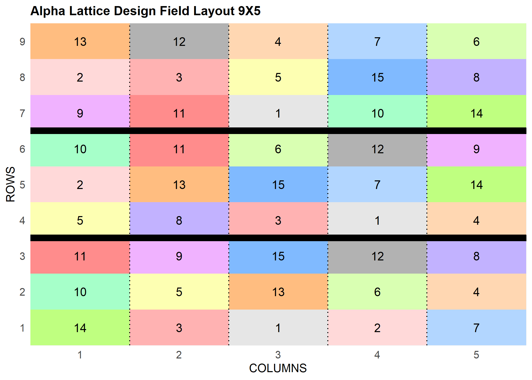
The alpha_lattice() function only runs when the number of treatments factorises into block size times blocks per replicate (\(v = sk\)); if the numbers do not fit, it reports which constraints were violated. That check alone is a good reason to use a dedicated package rather than writing the randomization by hand.
The agricolae equivalent
For users already familiar with {agricolae}, the same CRD can be generated with a single call:
crd_agri <- design.crd(
  trt  = paste0("T", 1:4),
  r    = 5,
  seed = 42
)

crd_agri$book %>% head()
plots r paste0("T", 1:4)
1 101 1 T1
2 102 1 T2
3 103 1 T4
4 104 2 T1
5 105 2 T4
6 106 1 T3The output is a data frame rather than a ready-made plot, which is convenient when the randomization is only one step in a larger pipeline (e.g. when it is merged with a data collection sheet or uploaded to a field management system).
A hand-drawn field map with ggplot2
Regardless of which package generates the randomization, a short ggplot2 recipe turns the field book into a customizable layout plot. The example below uses the RCBD generated above:
field_df <- rcbd_out$fieldBook %>%
  group_by(REP) %>%
  mutate(
    col = row_number(),
    plot_label = glue("P{PLOT}\n{TREATMENT}")
  ) %>%
  ungroup()

ggplot(field_df, aes(x = col, y = REP, fill = TREATMENT)) +
  geom_tile(colour = "white", linewidth = 1) +
  geom_text(aes(label = plot_label), size = 3) +
  scale_y_reverse(breaks = unique(field_df$REP)) +
  coord_equal() +
  labs(
    title = "RCBD layout (6 treatments, 4 complete blocks)",
    x = "Position within block",
    y = "Block (REP)",
    fill = "Treatment"
  ) +
  theme_minimal()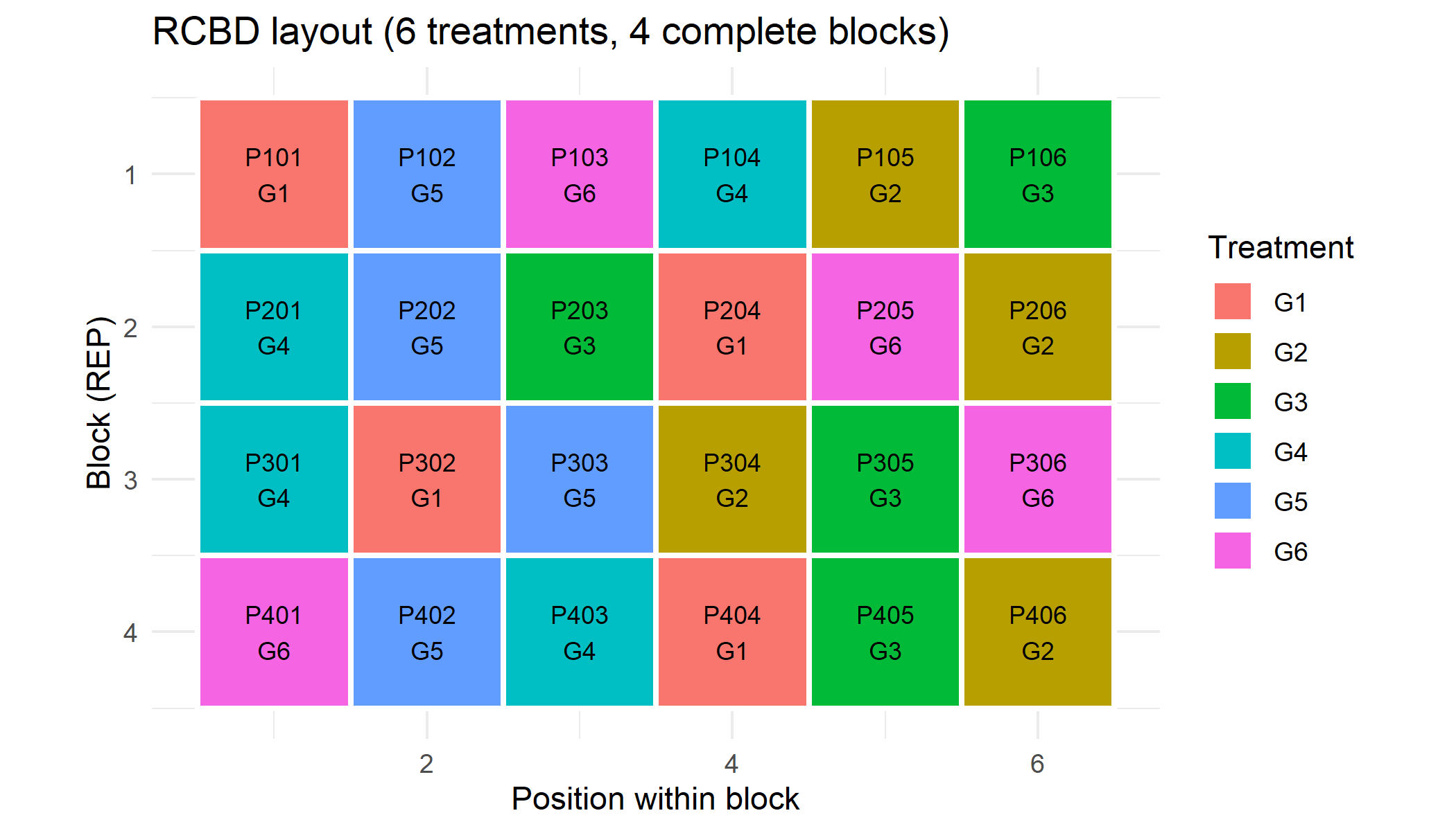
This recipe scales to any of the designs generated by FielDHub because they all return a $fieldBook with the same columns. Adapting the plot — adding block borders, highlighting checks, or rendering multiple environments as facets — is then a matter of standard ggplot2.
Practical Tips
A few points come up repeatedly in real trials and deserve a brief mention.
Border effects
Plots at the edge of a field, tray, or plate behave differently from plots in the interior: they receive more light, experience more wind, or are more accessible to pests. Ignoring this edge effect can bias the treatment means of anything placed on the border. Two common countermeasures:
- Add an unharvested guard row or guard column around the whole experiment (and sometimes between blocks). The guard material is usually a single check or a filler variety and is not analysed.
- Explicitly model row and column effects (see Chapter 6), which absorbs some of the spatial gradient regardless of where on the field a treatment was placed.
Repeated checks
Even in designs where most entries are not replicated (augmented, p-rep), a small set of well-known check varieties is usually included and replicated across the whole experiment. These checks serve two purposes: they anchor the analysis by providing a reference point in each block, and they allow the experimenter to monitor unusual conditions (if a normally stable check behaves strangely in one block, that block is suspect).
Seed values and reproducibility
All functions shown above take a seed argument. Recording the seed together with the field book is mandatory for reproducibility — without it, a re-run cannot produce the exact same randomization. In series of trials across multiple environments, each environment should use a different seed so that spatial patterns are not inadvertently copied from one site to the next.
Randomize, then check the layout
A generated randomization is not automatically a sensible randomization. Before the experiment starts, the layout should be inspected visually: Are any two treatments always next to each other? Is a single treatment stuck in the corner? Did the random number generator produce a pattern that happens to align with a known gradient? If anything looks wrong, simply change the seed and generate a new layout — that is cheap and legitimate, as long as the decision is made before data are collected.
Further Reading
For a deeper treatment of the topics covered here:
- General principles and philosophy — Fisher’s The Design of Experiments (1935) is the original source; a highly readable modern alternative is Cochran & Cox, Experimental Designs (2nd ed., Wiley, 1957), which remains the reference handbook for practical layouts.
- Agronomic focus — Casler (2015) gives a concise, hands-on overview of the three fundamental principles with agricultural examples.
- Multi-environment trials — H. P. Piepho, Büchse, and Emrich (2003) and H. P. Piepho, Büchse, and Richter (2004) describe the statistical framework for series of trials, including how to combine information across sites and years.
- Modern p-rep and partially replicated designs — Hans-Peter Piepho et al. (2022) covers resource-efficient alternatives to full replication that have become standard in plant breeding.
-
Software — the FielDHub and
{agricolae}package vignettes are the most practical starting point for generating any of the designs mentioned above.
- Design before data. The design must be chosen and generated before the experiment starts; no statistical method can fix a bad design after the fact.
- Replication, randomization, local control — Fisher’s three principles remain the foundation of any sound design.
- Let the constraints choose the design. Number of treatments, heterogeneity of the material, and available resources usually narrow the choice to one or two options.
-
Use a package. FielDHub and
{agricolae}cover nearly all designs encountered in practice and eliminate whole classes of hand-coded errors. - Record the seed. The randomization is part of the experiment and must be reproducible.
- Inspect the layout visually before starting the experiment. If it looks wrong, regenerate it.
References
Citation
@online{schmidt2026,
  author = {{Dr. Paul Schmidt}},
  title = {A7. {Designing} {Experiments}},
  date = {2026-06-08},
  url = {https://biomathcontent.netlify.app/content/lin_mod_exp/a7_designing.html},
  langid = {en}
}