A5. Compact Letter Display (CLD)

To install and load all the packages used in this chapter, run the following code:

for (pkg in c("emmeans", "multcomp", "multcompView", "ggtext", "scales", "tidyverse")) {
  if (!require(pkg, character.only = TRUE)) install.packages(pkg)
}

library(emmeans)
library(multcomp)
library(multcompView)
library(ggtext)
library(scales)
library(tidyverse)

A Compact Letter Display (CLD) is a popular way to summarise the results of all pairwise comparisons among treatment means. Each mean is annotated with one or more letters, and the rule is simple: means that do not share a letter are significantly different. The underlying algorithm was formalised by H. P. Piepho, Büchse, and Richter (2004), and its interpretation was carefully revisited by Hans-Peter Piepho (2018).

This chapter covers how to produce a CLD in R using emmeans (the recommended modern workflow), how to embed the letters in a ggplot2 figure, and how to interpret and report CLDs responsibly. We assume you are already familiar with multiplicity adjustments as discussed in the preceding chapter on multiple comparisons.

The Quick Version

We use the built-in PlantGrowth dataset throughout. The workflow is always the same: fit a model, compute estimated marginal means with emmeans(), and pass those to cld().

mod <- lm(weight ~ group, data = PlantGrowth)

mod_means <- emmeans(mod, specs = "group")

mod_means_cld <- cld(mod_means,
                     adjust = "Tukey",
                     Letters = letters,
                     alpha = 0.05)

Note: adjust = "tukey" was changed to "sidak"
because "tukey" is only appropriate for one set of pairwise comparisons

mod_means_cld

 group emmean    SE df lower.CL upper.CL .group
 trt1    4.66 0.197 27     4.16     5.16  a    
 ctrl    5.03 0.197 27     4.53     5.53  ab   
 trt2    5.53 0.197 27     5.02     6.03   b   

Confidence level used: 0.95 
Conf-level adjustment: sidak method for 3 estimates 
P value adjustment: tukey method for comparing a family of 3 estimates 
significance level used: alpha = 0.05 
NOTE: If two or more means share the same grouping symbol,
      then we cannot show them to be different.
      But we also did not show them to be the same. 

The .group column carries the letters. Here, trt1 shares no letter with trt2, so these two means differ significantly at the 5% level. ctrl shares letters with both, so we cannot distinguish it from either.

TipWhich cld() are we calling?

There are two cld() implementations in the R ecosystem: one in multcomp (for glht objects) and the method for emmGrid objects provided by multcomp via emmeans. Loading both packages makes the dispatch automatic. The old direct call multcomp::cld(glht(...)) still works but is no longer the recommended entry point – emmeans::emmeans() %>% cld() is more flexible, works for mixed models, and honours multiplicity adjustments transparently.

The Arguments That Matter

The three arguments you will tune most often are adjust, Letters and alpha.

• adjust controls the multiplicity adjustment ("tukey", "bonferroni", "sidak", "none", …). See the chapter on multiple comparisons (A4) for the theory.
• Letters = letters forces the output to use a-z. The default is numeric, which is rarely what you want from something called a letter display.
• alpha sets the significance threshold for deciding whether two means get separate letters.

NoteA confusing but harmless message

You may see a note like:

## Note: adjust = "tukey" was changed to "sidak"
## because "tukey" is only appropriate for one set of pairwise comparisons

This is not an error. The pairwise p-values are still Tukey-adjusted; only the confidence intervals on the means themselves fall back to the Sidak adjustment because Tukey is defined for contrasts, not single means. Background: stats.stackexchange.com.

Plotting the CLD

Putting the letters on a plot is the most common follow-up question. The pattern is:

1. Convert the cld() output to a tibble.
2. Trim whitespace in .group (cld() pads the letters for alignment).
3. Map the cleaned letters to a text layer.

mod_means_cld_tbl <- mod_means_cld %>%
  as_tibble() %>%
  mutate(.group = str_trim(.group)) %>%
  mutate(group = fct_reorder(group, emmean))

ggplot(mod_means_cld_tbl, aes(x = group, y = emmean)) +
  geom_point(size = 2) +
  geom_errorbar(aes(ymin = lower.CL, ymax = upper.CL), width = 0.1) +
  geom_text(aes(label = .group), nudge_x = 0.15, hjust = 0) +
  scale_y_continuous(
    name = "Mean weight with 95% CI",
    limits = c(0, NA),
    breaks = pretty_breaks(),
    expand = expansion(mult = c(0, 0.05))
  ) +
  scale_x_discrete(name = NULL, labels = str_to_title) +
  labs(caption = "Means not sharing a letter differ significantly (Tukey, alpha = 0.05).") +
  theme_classic() +
  theme(plot.caption = element_textbox_simple(hjust = 1))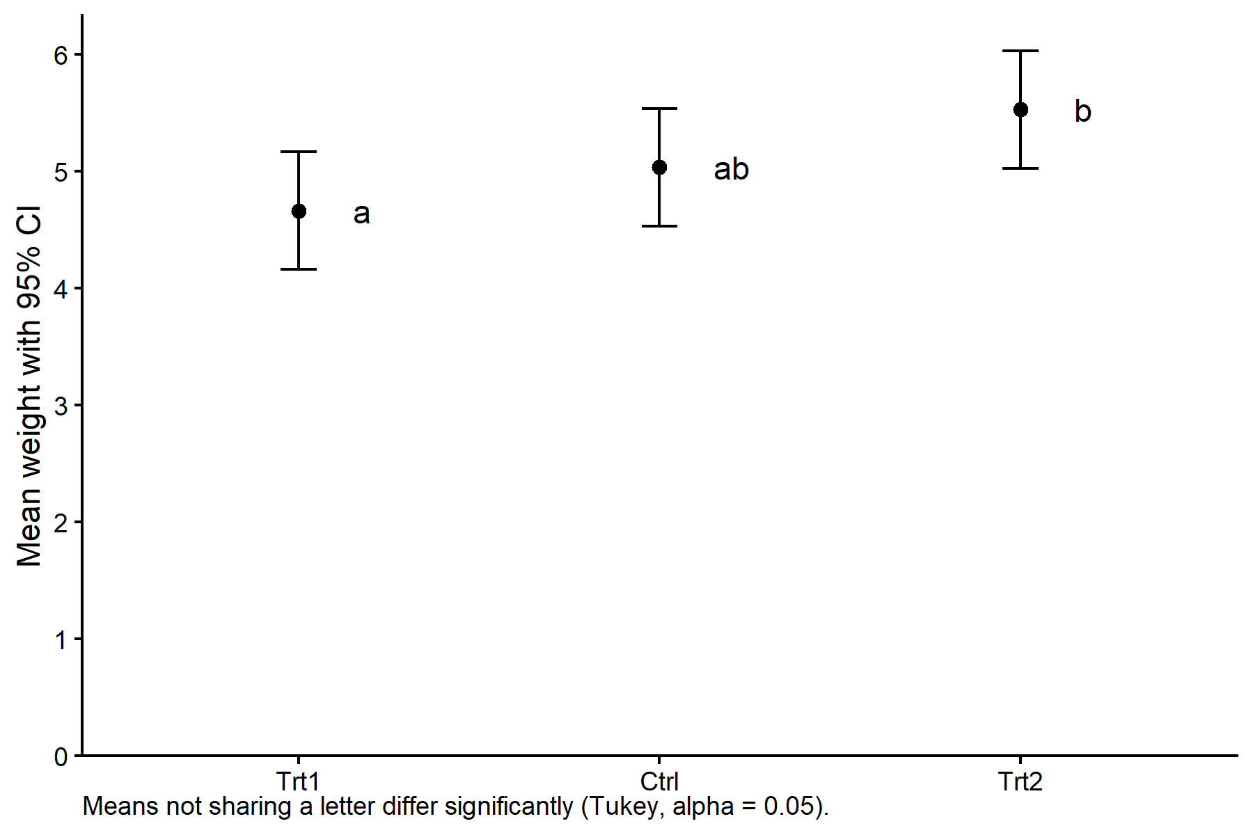

For more sophisticated styling (fonts, colour palettes, theme components) see the chapters in the ggplot2 section of this site.

A Richer Plot

The minimal plot above summarises the model output. Sometimes it is worth showing the raw data alongside the estimated means so readers can judge both the effect size and the data quality in one glance:

PlantGrowth2 <- PlantGrowth %>%
  mutate(group = fct_relevel(group, levels(mod_means_cld_tbl$group)))

ggplot() +
  geom_point(data = PlantGrowth2,
             aes(x = group, y = weight),
             shape = 16, alpha = 0.5,
             position = position_nudge(x = -0.2)) +
  geom_boxplot(data = PlantGrowth2,
               aes(x = group, y = weight),
               width = 0.05, outlier.shape = NA,
               position = position_nudge(x = -0.1)) +
  geom_point(data = mod_means_cld_tbl,
             aes(x = group, y = emmean),
             size = 2, color = "red") +
  geom_errorbar(data = mod_means_cld_tbl,
                aes(x = group, ymin = lower.CL, ymax = upper.CL),
                width = 0.05, color = "red") +
  geom_text(data = mod_means_cld_tbl,
            aes(x = group, y = emmean, label = .group),
            nudge_x = 0.1, hjust = 0, color = "red") +
  scale_y_continuous(name = "Weight",
                     limits = c(0, NA),
                     breaks = pretty_breaks(),
                     expand = expansion(mult = c(0, 0.1))) +
  scale_x_discrete(name = "Treatment") +
  labs(caption = glue::glue(
    "Black: raw data and boxplot. Red: estimated marginal means with 95% CI. ",
    "Means not sharing a letter differ significantly (Tukey, alpha = 0.05)."
  )) +
  theme_classic() +
  theme(plot.caption = element_textbox_simple())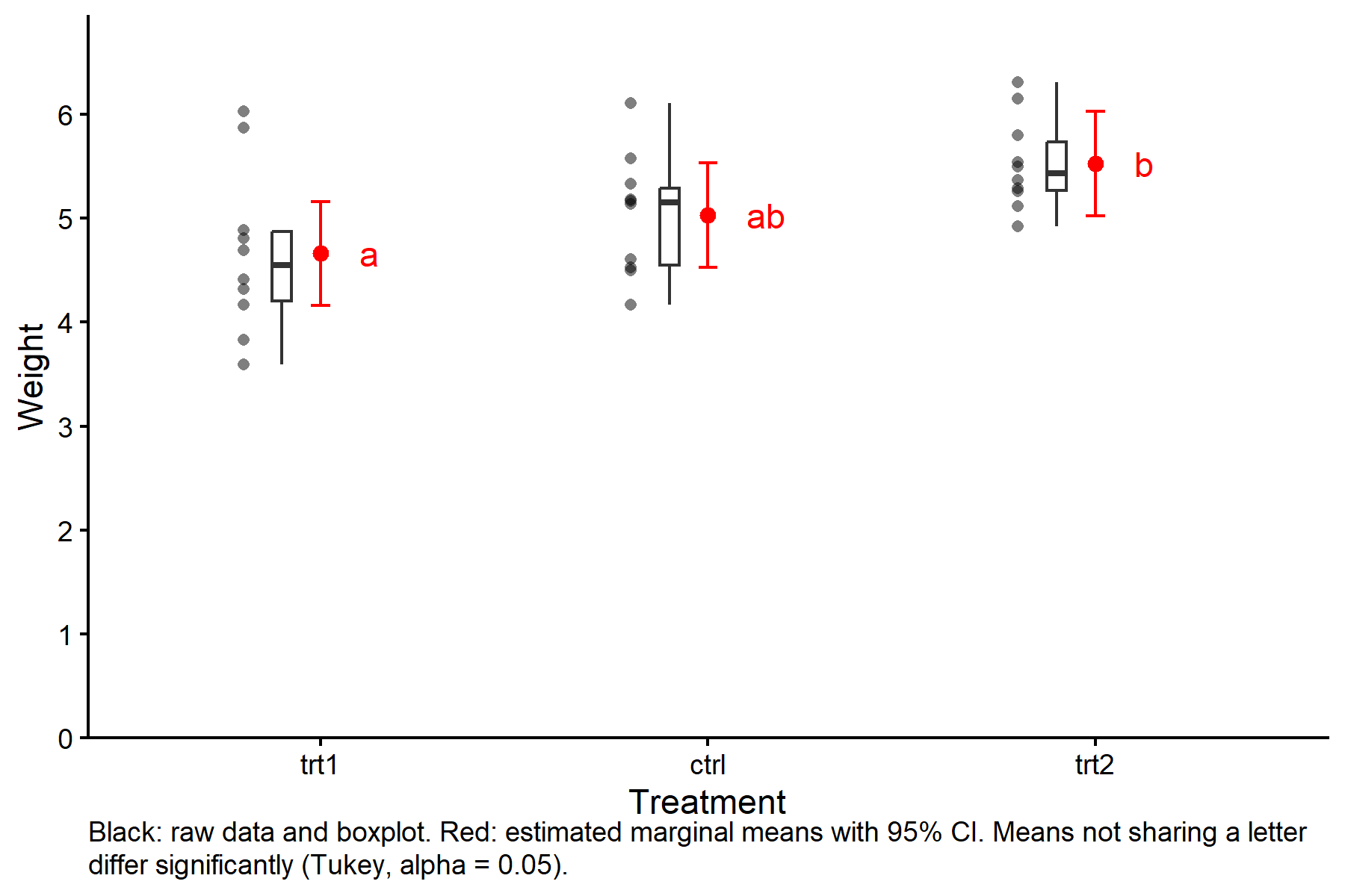

Bar plots with error bars (“dynamite plots”) are another traditional choice, but they hide the underlying distribution and are generally discouraged in modern data visualisation.

Interpreting CLDs Carefully

CLDs are convenient, but they come with a well-documented pitfall: they report non-findings, not findings. Two means sharing a letter does not prove that they are equal – it only means the test failed to reject equality. Hans-Peter Piepho (2018) makes this point explicitly and recommends a single, unambiguous caption:

Means not sharing any letter are significantly different at the chosen significance level.

Avoid wording like “means with the same letter are equal” or “means with the same letter do not differ.” Both overstate what the letters actually tell us.

ImportantRussell Lenth’s warning

The maintainer of emmeans, Russell V. Lenth, has been outspoken about the limitations of CLDs. Two common critiques:

• Black-and-white thresholding. A p-value of 0.049 and 0.051 are practically identical, yet a CLD treats them as opposites.
• Obscuring effect sizes. The letters collapse a rich set of pairwise comparisons into a single categorical summary.

The package even used to print the note “Compact letter displays can be misleading because they show NON-findings rather than findings.” The current wording is milder but carries the same message: “If two or more means share the same grouping letter, then we cannot show them to be different. But we also did not show them to be the same.” See Lenth’s commentary on Cross Validated.

If you want to communicate effect sizes more transparently, consider showing the pairwise comparisons directly (next section) in addition to, or instead of, the CLD.

Seeing the Underlying Comparisons

The letters are built from pairwise comparisons. To inspect those comparisons, use pairs() with infer = c(TRUE, TRUE) to get both confidence intervals and p-values:

mod_means %>%
  pairs(adjust = "tukey", infer = c(TRUE, TRUE))

 contrast    estimate    SE df lower.CL upper.CL t.ratio p.value
 ctrl - trt1    0.371 0.279 27    -0.32    1.062   1.331  0.3909
 ctrl - trt2   -0.494 0.279 27    -1.19    0.197  -1.772  0.1980
 trt1 - trt2   -0.865 0.279 27    -1.56   -0.174  -3.103  0.0120

Confidence level used: 0.95 
Conf-level adjustment: tukey method for comparing a family of 3 estimates 
P value adjustment: tukey method for comparing a family of 3 estimates 

Alternatively, passing details = TRUE to cld() returns both the letter display and the comparisons in one object:

cld(mod_means, adjust = "tukey", Letters = letters, details = TRUE)

Note: adjust = "tukey" was changed to "sidak"
because "tukey" is only appropriate for one set of pairwise comparisons

$emmeans
 group emmean    SE df lower.CL upper.CL .group
 trt1    4.66 0.197 27     4.16     5.16  a    
 ctrl    5.03 0.197 27     4.53     5.53  ab   
 trt2    5.53 0.197 27     5.02     6.03   b   

Confidence level used: 0.95 
Conf-level adjustment: sidak method for 3 estimates 
P value adjustment: tukey method for comparing a family of 3 estimates 
significance level used: alpha = 0.05 
NOTE: If two or more means share the same grouping symbol,
      then we cannot show them to be different.
      But we also did not show them to be the same. 

$comparisons
 contrast    estimate    SE df t.ratio p.value
 ctrl - trt1    0.371 0.279 27   1.331  0.3909
 trt2 - trt1    0.865 0.279 27   3.103  0.0120
 trt2 - ctrl    0.494 0.279 27   1.772  0.1980

P value adjustment: tukey method for comparing a family of 3 estimates 

Alternatives to the CLD

emmeans provides two visual alternatives that avoid the letter-display pitfalls:

pwpp(mod_means) + theme_bw()

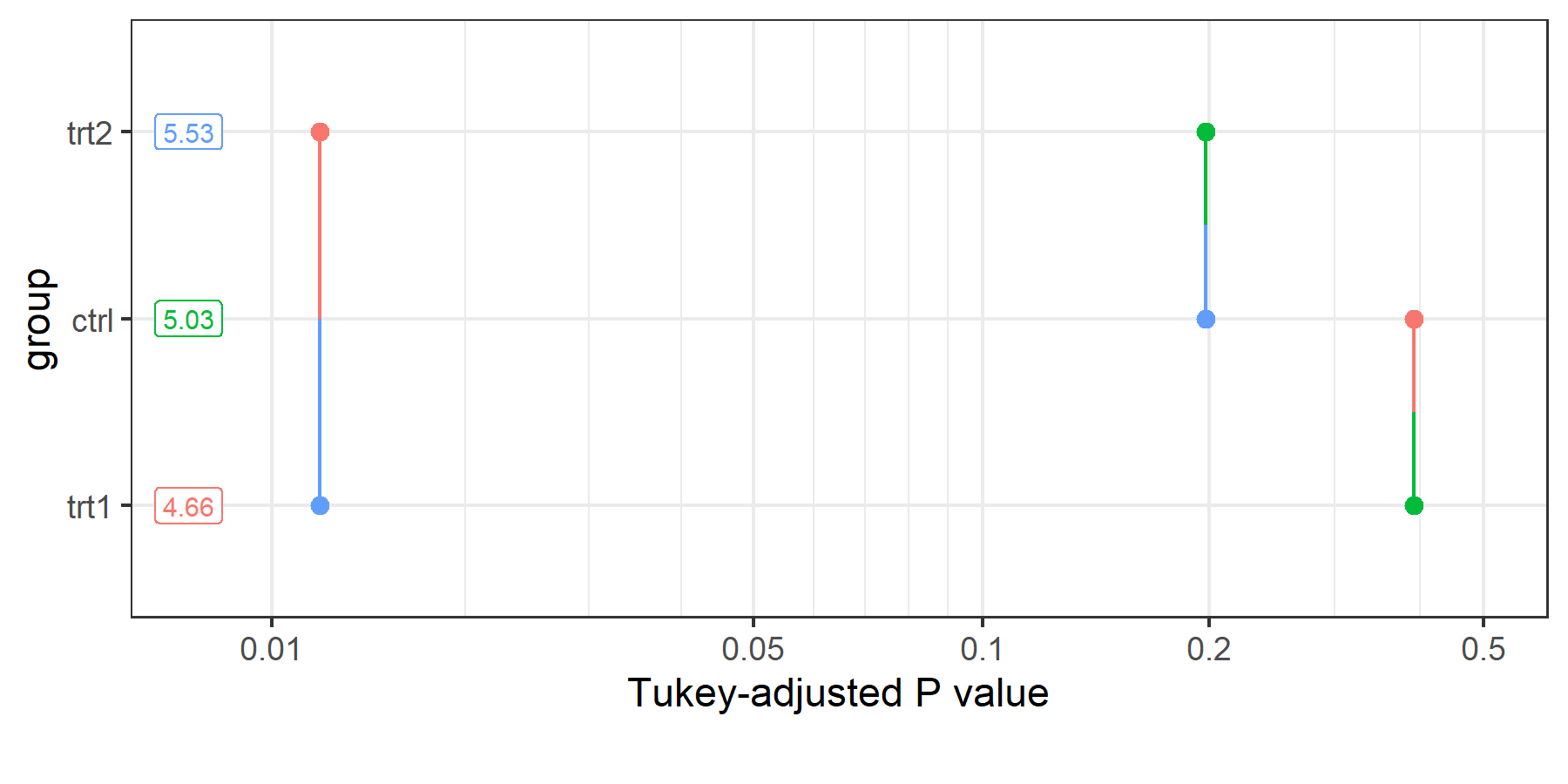
The pairwise p-value plot (pwpp()) shows every p-value on a horizontal axis and connects the two levels being compared with a line segment. This exposes p-values as a continuum rather than a binary significance decision.

The pairwise p-value matrix (pwpm()) prints a compact matrix with p-values above the diagonal and estimated differences below, and is useful in reports where a figure would be overkill.

When to Use (and Not Use) a CLD

A CLD is a pragmatic summary. It is appropriate when:

• You have a modest number of treatment levels (say, up to about ten).
• The audience expects or is familiar with letter-based summaries.
• A single table or plot needs to convey many comparisons at once.

It is less suitable when:

• Effect sizes matter more than a yes/no significance verdict (show confidence intervals).
• The number of means is large – the letter code becomes hard to parse.
• The context is one where sharing a letter might be misread as “equivalent” rather than “not shown to differ.”

NoteKey Takeaways

1. Use emmeans() %>% cld() as the standard workflow. Set Letters = letters and pick an adjust method deliberately.
2. The letters encode non-findings, not findings. Caption plots accordingly.
3. CLDs complement, but do not replace, the underlying pairwise comparisons. pairs() and pwpp() remain valuable diagnostic tools.
4. Trim whitespace in .group before plotting, and prefer point-and-error-bar plots over bar plots for the letter annotation.

References

Piepho, H. P., A. Büchse, and C. Richter. 2004. “A Mixed Modelling Approach for Randomized Experiments with Repeated Measures.” Journal of Agronomy and Crop Science 190 (4): 230–47. https://doi.org/10.1111/j.1439-037X.2004.00097.x.

Piepho, Hans-Peter. 2018. “Letters in Mean Comparisons: What They Do and Don’t Mean.” Agronomy Journal 110 (2): 431–34. https://doi.org/10.2134/agronj2017.10.0580.