2. The Tidyverse

As we’ve covered the very basics in the last section, we are eager to finally handle actual tables and not just individual values and vectors. And indeed, this is what we will do now. However, this is also a good point to start talking about the Tidyverse.

The Tidyverse is not just one, but a collection of multiple R packages that work together and - simply put - make using R for all kinds of data handling easier, faster and more powerful at the same time. What follows are several comparisons of doing something with base R on one hand and with the Tidyverse on the other hand. You must realize that R can do all of those things without using functions and packages from the Tidyverse - after all R existed without the tidyverse packages for a long time. However, the Tidyverse is a very popular and powerful way of doing things and I am not the only one who prefers it over the base R way of doing things.

To install and load all the packages used in this chapter, run the following code:

# install packages (only if not already installed)
for (pkg in c("tidyverse")) {
  if (!require(pkg, character.only = TRUE)) install.packages(pkg)
}

# load packages
library(tidyverse)

Note that we get a quite long output when loading the package called Tidyverse. This is because the Tidyverse is not just one package, but a collection of multiple packages. The library(tidyverse) command loads all of them at once. This is a very convenient feature as we usually use multiple packages from the Tidyverse at the same time. Thus, in the first part of the output it simply lists all the 9 packages that were loaded. The second part about the conflicts will be discussed later.

TipTip

As you can see above, I have used a # not only to write comments, but also to “comment out” code. More specifically I have added a # in front of the install.packages("tidyverse") command, which means that this command is not run when you execute the code, but the code is easily available for you to run it if you need to.

This is a very useful feature in R and many other programming languages. If you want to run a command, but not right now, you can comment it out and run the rest of the code. Note that there is even a shortcut in RStudio to comment out code: After highlighting one or even multiple lines of code, press Ctrl + Shift + C to comment out the code. Press the same combination again to uncomment the code.

Tables

Table in base R: data.frame

For you, tables are likely the most important data structure in R. Often your data is stored in a .xlsx, .csv or similar file and you then read it into R. A table in R is referred to as a data.frame in base R terminology. Here is an example of how to create one yourself and save it in a variable called my_df:

(In practice you obviously you don’t often create tables manually as shown below. We will discuss importing data soon.)

my_df <- data.frame(
 name = c("Wei", "Priya", "Kwame", "Juan"),
 age = c(25, 30, 35, 28),
 height = c(180, 170, 190, 175)
)

my_df

   name age height
1   Wei  25    180
2 Priya  30    170
3 Kwame  35    190
4  Juan  28    175

As you can see, we used a function called data.frame() to create a table with three columns: name, age and height. Thus, these three do not work as predefined argument names like with the seq() function in the last section, but instead as the names of the columns to be created. Moreover, the content of each column is defined by a vector of length 4 so that ultimately a table with 3 columns and 4 rows is created.

Note that a data.frame really is a collection of vectors. This fact helps you understand how to work with tables in R. As a reminder: A vector is a collection of values of the same type. In the example above, the name column is a vector of character values, the age column is a vector of numeric values and the height column is a vector of numeric values as well. You can try to think about data you work with in your daily life and it is likely that each column contains values of the same type.

You have multiple options to access parts of a data.frame. For example, you can access a single column by using the $ operator. Doing so returns the individual vector that represents the column:

my_df$name

[1] "Wei"   "Priya" "Kwame" "Juan" 

You can also use the square brackets ([]) to extract certain parts of the table - just like we did with vectors in the last section. However, you have to remember that a table is two-dimensional and thus you have to specify both the row and the column you want to access. You can do this by using the [row, column] syntax. For example, to access the age of the second person in the table, you can use:

my_df[2, "age"] # alternatively: my_df[2, 2] since age is the second column

[1] 30

Finally, here are two functions that you typically find in every R tutorial to investigate the structure of a table:

str(my_df)

'data.frame':   4 obs. of  3 variables:
 $ name  : chr  "Wei" "Priya" "Kwame" "Juan"
 $ age   : num  25 30 35 28
 $ height: num  180 170 190 175

First, we see that the data.frame has 4 observations (=rows) of 3 variables (=columns). Then, we get a sort of overview of each column telling us their names, data types and the first few values (in this case all values).

summary(my_df)

     name                age            height     
 Length:4           Min.   :25.00   Min.   :170.0  
 Class :character   1st Qu.:27.25   1st Qu.:173.8  
 Mode  :character   Median :29.00   Median :177.5  
                    Mean   :29.50   Mean   :178.8  
                    3rd Qu.:31.25   3rd Qu.:182.5  
                    Max.   :35.00   Max.   :190.0  

This function also provides information about the columns of the table, but in a different way. For example: for numeric columns, it gives you the minimum, 1st quartile, median, mean, 3rd quartile and maximum value.

Table in the Tidyverse: tibble

Everything you have seen so far is the base R way of handling tables. Now, let’s see how the Tidyverse does it. The Tidyverse has its own table structure called tibble. According to the authours the tibble “is a modern reimagining of the data.frame, keeping what time has proven to be effective, and throwing out what is not.” In other words, the tibble is a bit more user-friendly and has some advantages over the data.frame. Note that it is not a completely separate data structure, but rather a modified version of - and still based on - the data.frame.

Before we can work with tibbles we must install and load the required package - which we did at the beginning of this chapter. If you scroll up to the list of packages that was shown when loading the tidyverse, you’ll notice that one of them was called tibble. This is the package that provides the tibble data structure and all the functions that come with it.

Here is how we would create the same table as above, but this time as a tibble and save it in a variable called my_tbl:

my_tbl <- tibble(
 name = c("Wei", "Priya", "Kwame", "Juan"),
 age = c(25, 30, 35, 28),
 height = c(180, 170, 190, 175)
)

my_tbl

# A tibble: 4 × 3
  name    age height
  <chr> <dbl>  <dbl>
1 Wei      25    180
2 Priya    30    170
3 Kwame    35    190
4 Juan     28    175

Note that regarding the code, there really is only one difference to the base R way of creating a table: We use the tibble() function instead of the data.frame() function. However, the output is a bit different and this is where the advantages of the tibble come into play. While it is still the same table in terms of its content, the tibble is automatically printed in a more user-friendly way. Here is an example of a tibble with 153 rows, 12 columns, missing values NA and negative values:

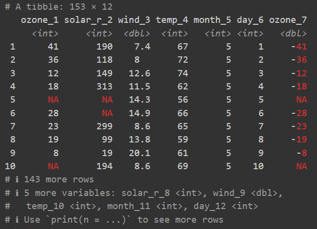
1. There is an extra first line telling us about the number of rows and columns.
2. There is an extra line below the column names telling us about the data type of each column.
3. Only the first ten rows of data are printed.
4. Only the first columns of data are printed.
5. Missing values NA and negative numbers are printed in red.

All of these small things really add up over time and make working with tibbles more pleasant than with data.frames. Finally, note that in its heart, a tibble is still a data.frame and in most cases you can do everything with a tibble that you can do with a data.frame. Here are the same commands we used above as proof:

my_tbl$name

[1] "Wei"   "Priya" "Kwame" "Juan" 

str(my_tbl)

tibble [4 × 3] (S3: tbl_df/tbl/data.frame)
 $ name  : chr [1:4] "Wei" "Priya" "Kwame" "Juan"
 $ age   : num [1:4] 25 30 35 28
 $ height: num [1:4] 180 170 190 175

summary(my_tbl)

     name                age            height     
 Length:4           Min.   :25.00   Min.   :170.0  
 Class :character   1st Qu.:27.25   1st Qu.:173.8  
 Mode  :character   Median :29.00   Median :177.5  
                    Mean   :29.50   Mean   :178.8  
                    3rd Qu.:31.25   3rd Qu.:182.5  
                    Max.   :35.00   Max.   :190.0  

Therefore, there basically is no downside and instead only advantages to using tibbles over data.frames. And what is true here for tables also exemplifies the general idea of the Tidyverse: It is not necessarily a completely new way of doing things, but rather a more user-friendly and powerful way of doing things that were already possible before.

NoteAdditional Resources

At this point I would like to recommend a free, oline book that is a great resource for learning the Tidyverse and R in general: “R for Data Science (2e)”. It was written by Hadley Wickham, Mine Çetinkaya-Rundel, and Garrett Grolemund, which are themselves authors of some of the most important Tidyverse packages.

A new example dataset

Before we continue, let us get rid of the small tables we created above and instead use a built-in dataset that comes with R. This dataset is called PlantGrowth and contains data on the weight of 30 plants in 3 different groups. As it is built-in (just like pi; see last chapter) we can access it directly by its name. However, it is a data.frame and I would like to work with a tibble instead. Therefore, I will convert it to a tibble using the as_tibble() function and save it into a variable called tbl:

tbl <- as_tibble(PlantGrowth)

tbl

# A tibble: 30 × 2
   weight group
    <dbl> <fct>
 1   4.17 ctrl 
 2   5.58 ctrl 
 3   5.18 ctrl 
 4   6.11 ctrl 
 5   4.5  ctrl 
 6   4.61 ctrl 
 7   5.17 ctrl 
 8   4.53 ctrl 
 9   5.33 ctrl 
10   5.14 ctrl 
# ℹ 20 more rows

Note that you can now for the first time see the tibble functionality in action where it does not flood the output with all 30 rows of data, but instead only shows the first 10 rows and adds a “… with 20 more rows” below. This is a very useful feature when working with large datasets.

Plots

Plot in base R: plot()

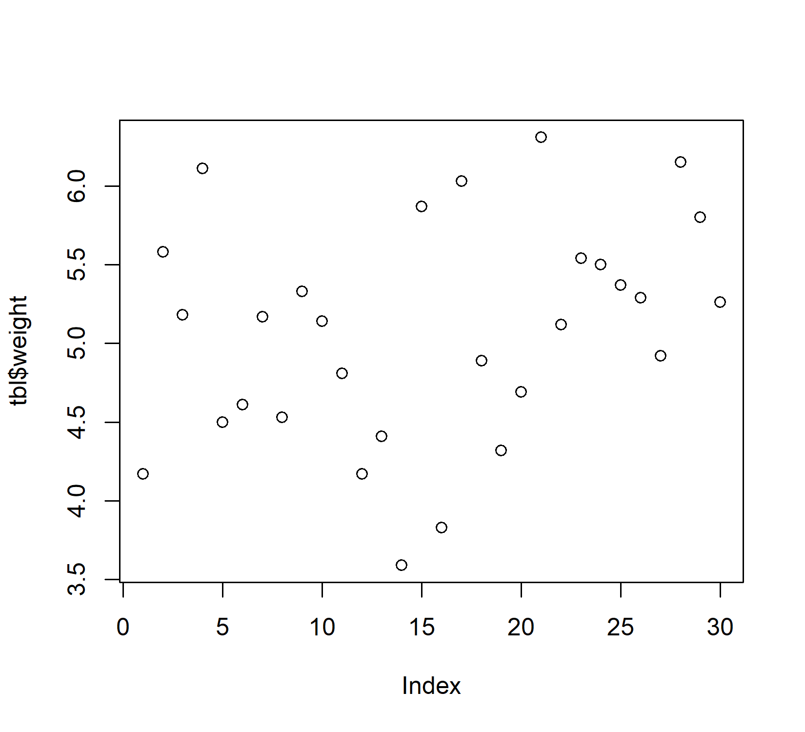
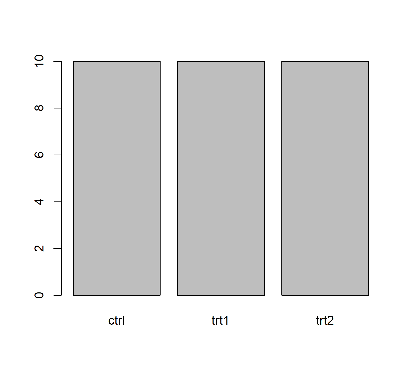
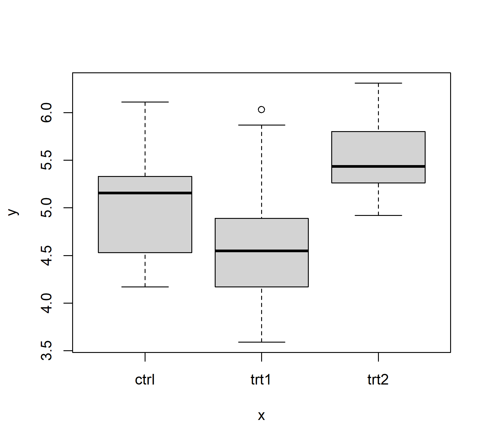
Base R has a plot() function which is good at getting some first data visualizations with very little code. It guesses what type of plot you would like to see via the data type of the respective data to be plotted:

plot(tbl$weight) # scatter plot of values in the order they appear
plot(tbl$group) # bar plot of frequency of each level
plot(x = tbl$group, y = tbl$weight) # boxplot for values of each level

Plot in the Tidyverse: ggplot()

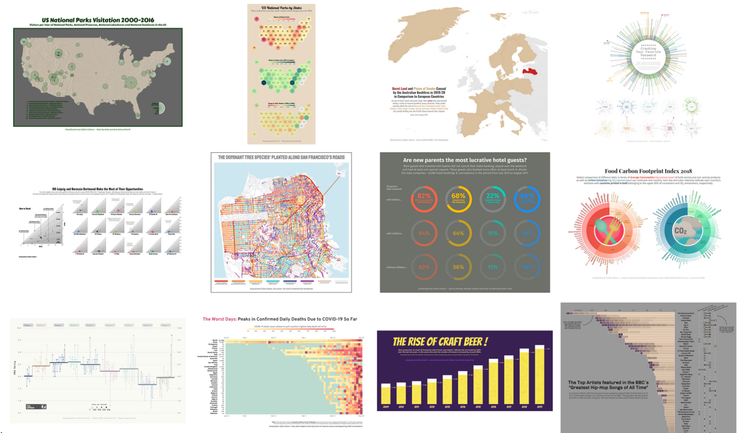
However, I really just use plot() to get a quick first glance at data. In order to get professional visualizations I always use the tidyverse package ggplot2 and its function ggplot(). It seems like it can create any plot you can imagine. However, its high capability comes with the price of a long learning curve. Therefore, I only refer to additional resources for now and will cover some basics in the next sections. Yet, as an appetizer, here is a screenshot of some plots created with ggplot by Cédric Scherer:

NoteAdditional Resources

• How I use ggplot2
• ggplot2 extensions gallery

The pipe oprerator

The pipe operator (%>% or |>) “completely changed the way how we code in R, making it more simple and readable” (Álvarez, 2001). I started using the pipe as %>% from the {dplyr} package¹. However, since May 18, 2021 (= R 4.1.0) the pipe is officially part of Base R - although written as |>. Note that there are some differences between %>% and |> - find more about it e.g. here, here or here.

To understand what makes it so great we need to start using more than one function at a time. So far, we have only used functions individually. Yet, in real life you will often find yourself having to combine multiple functions.

As an example, say we have three numbers 1, 4 and 10 (i.e. a vector c(1, 4, 10)) and we want to (i) take their square root, then (ii) get the mean of those values and (iii) take the square root of that mean. Finally, we want to save the result in a variable called result.

TipExercise: Combining Multiple Functions

Before you continue reading, try achieving this with the knowledge you already have, i.e. without the pipe operator.

NoteSolution

See the following three sections for different approaches to solve this problem.

Solution 1: Intermediate results

One way of achieving our goal here is do it step by step and save each intermediate result in a variable. This is a very common approach in programming and is called “stepwise” or “iterative” approach. Here is how it would look like in R:

x <- c(1, 4, 10)
step1 <- sqrt(x) # Step 1: Take the square root
step2 <- mean(step1) # Step 2: Get the mean
result <- sqrt(step2) # Step 3: Take the square root of the mean
result

[1] 1.433211

This works perfectly fine and it is easy to read, since we can see each step. However, it is also takes quite some code and creates variables that we do not really care about.

Solution 2: Nested functions

Another way of achieving the same result is to use nested functions - just like you would in Microsoft Excel. This means that we put one function inside another function:

x <- c(1, 4, 10)
result <- sqrt(mean(sqrt(x)))
result

[1] 1.433211

The obvious advantage is that it takes less code and does not create unnecessary variables. However, it is also less readable, because you have to read from the inside out. This is not a problem for simple functions like this one, but it can get very confusing with more complex functions.

Solution 3: The pipe operator

This combines the advantages of both approaches above, as it (i) allows you to write functions from left to right / top to bottom and thus in the order they are executed and the way you think about them and (ii) does not create extra variables for intermediate steps:

x <- c(1, 4, 10)
result <- x %>% sqrt() %>% mean() %>% sqrt()
result

[1] 1.433211

You can think about it like this: Something (in this case x) goes into the pipe and is directed to the next function sqrt(). By default, this function takes what came out of the previous pipe and puts it as its first argument. This happens with every pipe.

Maybe it helps to realize that these two do identical things:

• sqrt(9)
• 9 %>% sqrt()

TipTip

The keyboard shortcut for writing %>% in RStudio is CTRL+SHIFT+M. Keyboard shortcuts can be customized in RStudio as described here.

dplyr Verbs

We now have an idea how creating tables, plots and generally coding is nicer when using the Tidyverse. Another very important part of the Tidyverse is the package dplyr. This package provides a set of functions that are very useful for data manipulation. These functions are often referred to as “verbs” because they describe what you want to do with your data. Taken directly from the documentation:

{dplyr} is a grammar of data manipulation, providing a consistent set of verbs that help you solve the most common data manipulation challenges:

• mutate() adds new variables that are functions of existing variables.

• select() picks variables based on their names.

• filter() picks cases based on their values.

• summarise() reduces multiple values down to a single summary.

• arrange() changes the ordering of the rows.

These all combine naturally with group_by() which allows you to perform any operation “by group”. If you are new to dplyr, the best place to start is the data transformation chapter in R for data science.

In my experience you really can do most of the data manipulation before and after the actual statistics with these functions. In other words, it is exactly these functions who can and should replace the manual work you may currently be doing in MS Excel to handle your data. In the following sections I will give very brief examples of how to use these functions while always pointing to more thorough resources.

Before we start using them, let’s create some toy datasets that are nice to work with. Please ignore that we have not introduced some of the functions used below yet. We will cover them in the next sections. For now, we just want to create these four datasets to work with:

dat1 <- as_tibble(PlantGrowth)
dat2 <- dat1 %>% head() # keep first 6 rows
dat3 <- dat1 %>% slice(1:4, 11:14, 21:24) # keep rows 1-4, 11-14 and 21-24
dat4 <- dat1 %>% slice(1, 2, 11, 12, 21, 22) %>% # keep rows 1, 2, 11, 12, 21 and 22
  mutate(var1 = 1:6, var2 = 22:27, var3 = 3:8, var4 = 4:9)

NoteNote

Here is something that must be realized before we continue.

What you see above is code that created 4 new datasets/objects/variables (dat1 - dat3), each by taking a different dataset and manipulating it in some way. The first dataset is the built-in dataset PlantGrowth but formatted as a tibble. The reason why the manipulated version (i.e. the tibble version of PlantGrowth) is permanently available as dat1 is because we used the <- operator and saved that manipulated version in that new variable called dat1. Note further that we do not actually see these new datasets. If we wanted to see dat1, we would have to run dat1 (or print(dat1)) so that its content is printed to the console.

In the following sections we will do a loooot of data manipulations, because that’s what we will learn. However, we will actually never save the manipulated datasets into new variables. Instead, we will run the code without the ... <- and thus always simply print the manipulated version of the dataset to the console. This is good for the purpose of seeing what a function does. Yet it is obviously not what you will do in real life. In real life you will always save the manipulated version of the dataset into a new variable.

select()

The select() function allows you to select certain columns from a table. This is very useful when you have a large table and only want to work with a few columns. So this is our dataset:

dat4

# A tibble: 6 × 6
  weight group  var1  var2  var3  var4
   <dbl> <fct> <int> <int> <int> <int>
1   4.17 ctrl      1    22     3     4
2   5.58 ctrl      2    23     4     5
3   4.81 trt1      3    24     5     6
4   4.17 trt1      4    25     6     7
5   6.31 trt2      5    26     7     8
6   5.12 trt2      6    27     8     9

And when I use the select() function to select the column group, it will return a new table with only that column:

dat4 %>% select(group)

# A tibble: 6 × 1
  group
  <fct>
1 ctrl 
2 ctrl 
3 trt1 
4 trt1 
5 trt2 
6 trt2 

Moreover, you can name more than one column:

dat4 %>% select(group, var2, var4)

# A tibble: 6 × 3
  group  var2  var4
  <fct> <int> <int>
1 ctrl     22     4
2 ctrl     23     5
3 trt1     24     6
4 trt1     25     7
5 trt2     26     8
6 trt2     27     9

NoteNote

Once again a reminder that the pipe operator (%>%) is not strictly necessary here. The function select works by itself and it needs the data as its first argument. Thus, you could also write select(dat4, group) or select(dat4, group, var2, var4). However, we will continue using the pipe operator, because it makes the code easier to read and understand - at least in the long run.

You can even select multiple columns at once by using the : operator. For example, if you want to select all columns from var2 to var4, you can do this:

dat4 %>% select(group, var2:var4)

# A tibble: 6 × 4
  group  var2  var3  var4
  <fct> <int> <int> <int>
1 ctrl     22     3     4
2 ctrl     23     4     5
3 trt1     24     5     6
4 trt1     25     6     7
5 trt2     26     7     8
6 trt2     27     8     9

You can also use the - operator to exclude certain columns. For example, if you want to select all columns except var1, you can do this:

dat4 %>% select(-var1)

# A tibble: 6 × 5
  weight group  var2  var3  var4
   <dbl> <fct> <int> <int> <int>
1   4.17 ctrl     22     3     4
2   5.58 ctrl     23     4     5
3   4.81 trt1     24     5     6
4   4.17 trt1     25     6     7
5   6.31 trt2     26     7     8
6   5.12 trt2     27     8     9

Finally, there are several helper functions that allow you to select columns based on their names. For example, if you want to select all columns that start with “var”, you can use the helper function starts_with() like so:

dat4 %>% select(starts_with("var"))

# A tibble: 6 × 4
   var1  var2  var3  var4
  <int> <int> <int> <int>
1     1    22     3     4
2     2    23     4     5
3     3    24     5     6
4     4    25     6     7
5     5    26     7     8
6     6    27     8     9

Other, similar functions are ends_with(), contains(), matches() and num_range().

There are also functions like is.numeric(), is.character() etc. that allow you to select columns based on their data type. For example, if you want to select all numeric columns, you can do it like so:

dat4 %>% select(where(~is.numeric(.x)))

# A tibble: 6 × 5
  weight  var1  var2  var3  var4
   <dbl> <int> <int> <int> <int>
1   4.17     1    22     3     4
2   5.58     2    23     4     5
3   4.81     3    24     5     6
4   4.17     4    25     6     7
5   6.31     5    26     7     8
6   5.12     6    27     8     9

These are very powerful features of the select() function and allow you to select columns based on their names or data types without having to type them all out manually. Finally, there is even a helper function called everything(), which allows you to select all columns. This may not seem very useful at first, but you could e.g. use it to reorder columns by selecting specific columns first and then all other columns afterwards:

dat4 %>% select(var2, everything())

# A tibble: 6 × 6
   var2 weight group  var1  var3  var4
  <int>  <dbl> <fct> <int> <int> <int>
1    22   4.17 ctrl      1     3     4
2    23   5.58 ctrl      2     4     5
3    24   4.81 trt1      3     5     6
4    25   4.17 trt1      4     6     7
5    26   6.31 trt2      5     7     8
6    27   5.12 trt2      6     8     9

NoteAdditional Resources

• 5.4 Select columns with select() in R for data science
• Subset columns using their names and types with select()
• Select variables that match a pattern with starts_with() etc.
• Select variables with a function with where()

filter()

The filter() function allows you to filter rows based on certain conditions. You are probably familiar with this from Excel, where this is also called filtering.

In order to have something to filter from, we will use dat1 as it has 30 observations. In order to keep only those observations where the weight is greater than 6, we can use the filter() function like so:

dat1 %>% filter(weight > 6)

# A tibble: 4 × 2
  weight group
   <dbl> <fct>
1   6.11 ctrl 
2   6.03 trt1 
3   6.31 trt2 
4   6.15 trt2 

You can add a second condition by using the & operator to make it so that both condition 1 AND condition 2 must be true. For example, if you want to keep only those observations where the weight is greater than 6 AND the group is “trt2”, you can do this:

dat1 %>% filter(weight > 6 & group == "trt2")

# A tibble: 2 × 2
  weight group
   <dbl> <fct>
1   6.31 trt2 
2   6.15 trt2 

If you are confused why we need to write == instead of =, go back to the “Comparison Operators” section in the previous chapter and also remember that a single = is used for assigning values to variables. However, here we are not assigning anything, but rather checking if the value of group is equal to “trt2”. Thus, we need to use the double == operator.

You can also use the | operator to make it so that either condition 1 OR condition 2 must be true. For example, we could keep only those observations where the weight is greater than 6 OR smaller than 4:

dat1 %>% filter(weight > 6 | weight < 4)

# A tibble: 6 × 2
  weight group
   <dbl> <fct>
1   6.11 ctrl 
2   3.59 trt1 
3   3.83 trt1 
4   6.03 trt1 
5   6.31 trt2 
6   6.15 trt2 

The next three examples will all lead to the same result, but achieve it in different ways. It is almost always the case that there is not just a single way to do something in R, but sometimes one way is more efficient or easier to read than another. Our goal for all of them is to keep all observations that do not belong to the control group.

We could do it with the | operator we just learned about:

dat1 %>% filter(group == "trt1" | group == "trt2")

# A tibble: 20 × 2
   weight group
    <dbl> <fct>
 1   4.81 trt1 
 2   4.17 trt1 
 3   4.41 trt1 
 4   3.59 trt1 
 5   5.87 trt1 
 6   3.83 trt1 
 7   6.03 trt1 
 8   4.89 trt1 
 9   4.32 trt1 
10   4.69 trt1 
11   6.31 trt2 
12   5.12 trt2 
13   5.54 trt2 
14   5.5  trt2 
15   5.37 trt2 
16   5.29 trt2 
17   4.92 trt2 
18   6.15 trt2 
19   5.8  trt2 
20   5.26 trt2 

For situations where you would need to combine several more conditions, the %in% operator is a more efficient way of doing this. It allows you to check if a value is in a vector of values. For example, we could do the same as above like this:

dat1 %>% filter(group %in% c("trt1", "trt2"))

# A tibble: 20 × 2
   weight group
    <dbl> <fct>
 1   4.81 trt1 
 2   4.17 trt1 
 3   4.41 trt1 
 4   3.59 trt1 
 5   5.87 trt1 
 6   3.83 trt1 
 7   6.03 trt1 
 8   4.89 trt1 
 9   4.32 trt1 
10   4.69 trt1 
11   6.31 trt2 
12   5.12 trt2 
13   5.54 trt2 
14   5.5  trt2 
15   5.37 trt2 
16   5.29 trt2 
17   4.92 trt2 
18   6.15 trt2 
19   5.8  trt2 
20   5.26 trt2 

Finally, we could also use the != operator to check if the group is not equal to “ctrl”:

dat1 %>% filter(group != "ctrl")

# A tibble: 20 × 2
   weight group
    <dbl> <fct>
 1   4.81 trt1 
 2   4.17 trt1 
 3   4.41 trt1 
 4   3.59 trt1 
 5   5.87 trt1 
 6   3.83 trt1 
 7   6.03 trt1 
 8   4.89 trt1 
 9   4.32 trt1 
10   4.69 trt1 
11   6.31 trt2 
12   5.12 trt2 
13   5.54 trt2 
14   5.5  trt2 
15   5.37 trt2 
16   5.29 trt2 
17   4.92 trt2 
18   6.15 trt2 
19   5.8  trt2 
20   5.26 trt2 

In this specific case, the last of the three options is the shortest and easiest to read.

NoteAdditional Resources

• 5.2 Filter rows with filter() in R for data science
• Subset rows using column values with filter()

arrange()

The arrange() function allows you to arrange (i.e. sort) the rows of a table based on the values of one or more columns. Here we use dat3 which has 4 rows for each of the three groups:

dat3

# A tibble: 12 × 2
   weight group
    <dbl> <fct>
 1   4.17 ctrl 
 2   5.58 ctrl 
 3   5.18 ctrl 
 4   6.11 ctrl 
 5   4.81 trt1 
 6   4.17 trt1 
 7   4.41 trt1 
 8   3.59 trt1 
 9   6.31 trt2 
10   5.12 trt2 
11   5.54 trt2 
12   5.5  trt2 

We can sort the table by the weight column like this:

dat3 %>% arrange(weight)

# A tibble: 12 × 2
   weight group
    <dbl> <fct>
 1   3.59 trt1 
 2   4.17 ctrl 
 3   4.17 trt1 
 4   4.41 trt1 
 5   4.81 trt1 
 6   5.12 trt2 
 7   5.18 ctrl 
 8   5.5  trt2 
 9   5.54 trt2 
10   5.58 ctrl 
11   6.11 ctrl 
12   6.31 trt2 

As you can see, it is sorted ascendingly by default. If you want to sort it descendingly, you can use the desc() helper function and wrap it around the respective column name:

dat3 %>% arrange(desc(weight))

# A tibble: 12 × 2
   weight group
    <dbl> <fct>
 1   6.31 trt2 
 2   6.11 ctrl 
 3   5.58 ctrl 
 4   5.54 trt2 
 5   5.5  trt2 
 6   5.18 ctrl 
 7   5.12 trt2 
 8   4.81 trt1 
 9   4.41 trt1 
10   4.17 ctrl 
11   4.17 trt1 
12   3.59 trt1 

You can also sort by multiple columns. For example, you can first sort by group and then by weight. This works here, because of the duplicate values in the group column: The resulting table has the three groups in alphabetical order, but the rows within each group are sorted by weight:

dat3 %>% arrange(group, weight)

# A tibble: 12 × 2
   weight group
    <dbl> <fct>
 1   4.17 ctrl 
 2   5.18 ctrl 
 3   5.58 ctrl 
 4   6.11 ctrl 
 5   3.59 trt1 
 6   4.17 trt1 
 7   4.41 trt1 
 8   4.81 trt1 
 9   5.12 trt2 
10   5.5  trt2 
11   5.54 trt2 
12   6.31 trt2 

Note that here you could wrap group, weight or both in the desc() function as well, if you wanted to sort descendingly.

Finally, a slightly more advanced example would be to sort by a certain custom order. This is sometimes necessary, because you may not always want e.g. your groups in an alphabetical order (or reverse alphabetical order). Let’s pretend you want to sort by group in the order “trt2”, “ctrl”, “trt1”. We can achieve this by defining our custom order and making use of the helper function match():

myorder <- c("trt1", "ctrl", "trt2")

dat3 %>% arrange(match(group, myorder))

# A tibble: 12 × 2
   weight group
    <dbl> <fct>
 1   4.81 trt1 
 2   4.17 trt1 
 3   4.41 trt1 
 4   3.59 trt1 
 5   4.17 ctrl 
 6   5.58 ctrl 
 7   5.18 ctrl 
 8   6.11 ctrl 
 9   6.31 trt2 
10   5.12 trt2 
11   5.54 trt2 
12   5.5  trt2 

And of course you could even go on and e.g. sort weight within each group descendingly dat3 %>% arrange(match(group, myorder), desc(weight)).

NoteAdditional Resources

• 5.2 Filter rows with filter() in R for data science
• Subset rows using column values with filter()

mutate()

The mutate() function allows you to mutate (i.e. change) the values of existing columns or create new columns. Let’s again use dat2 which has only 6 rows and create a new column called “kg” that contains the weight in kilograms (i.e. assuming weight is in grams, so we divid by 1000):

dat2 %>% mutate(kg = weight / 1000)

# A tibble: 6 × 3
  weight group      kg
   <dbl> <fct>   <dbl>
1   4.17 ctrl  0.00417
2   5.58 ctrl  0.00558
3   5.18 ctrl  0.00518
4   6.11 ctrl  0.00611
5   4.5  ctrl  0.0045 
6   4.61 ctrl  0.00461

So as you can, mutate works by assigning (i.e. using =) a new column name (in this case kg) to the result of the operation (in this case dividing by 1000) on the existing column weight.

We could instead do the exact same operation but assign it to the column name weight. This will overwrite the existing column weight with the new values or in other words, it will mutate/change the existing column weight:

dat2 %>% mutate(weight = weight / 1000)

# A tibble: 6 × 2
   weight group
    <dbl> <fct>
1 0.00417 ctrl 
2 0.00558 ctrl 
3 0.00518 ctrl 
4 0.00611 ctrl 
5 0.0045  ctrl 
6 0.00461 ctrl 

We can also create multiple columns at once and they don’t need to be related to any of the existing columns:

dat2 %>%
  mutate(
    `Name with Space` = "Hello!",
    number10 = 10
  )

# A tibble: 6 × 4
  weight group `Name with Space` number10
   <dbl> <fct> <chr>                <dbl>
1   4.17 ctrl  Hello!                  10
2   5.58 ctrl  Hello!                  10
3   5.18 ctrl  Hello!                  10
4   6.11 ctrl  Hello!                  10
5   4.5  ctrl  Hello!                  10
6   4.61 ctrl  Hello!                  10

So here, two columns are created and simply filled with the same value for all rows. Note that the column name Name with Space contains spaces, which is not allowed in R. However, if you really want to, you can use backticks (`) to create column names with spaces or other special characters.

A bit more advanced, but very powerful is the combination of mutate() and case_when(). This allows you to create new columns based on conditions. In the following example we create a column named size that contains the values “large”, “small” or “normal” depending on the value of the weight column. If the weight is greater than 5.5, it is “large”, if it is smaller than 4.5, it is “small” and everything else is “normal”:

dat2 %>%
  mutate(size = case_when(
    weight > 5.5 ~ "large",
    weight < 4.5 ~ "small",
    TRUE ~ "normal" # everything else
  ))

# A tibble: 6 × 3
  weight group size  
   <dbl> <fct> <chr> 
1   4.17 ctrl  small 
2   5.58 ctrl  large 
3   5.18 ctrl  normal
4   6.11 ctrl  large 
5   4.5  ctrl  normal
6   4.61 ctrl  normal

Thus, you can see that the respective condition works the exact same way as for the filter() function. However, we then write a tilde (~) and the value we want to assign to the new column if the condition is true. These conditions are actually evaluated in the order they are written. This means that if the first condition is true, the second condition will not be evaluated. For this example this means that once a size is set to “large”, it wont be checked for the following conditions. Because of this behaviour, we can simply put a TRUE as the last condition, as it will simply be true for all remaining values and assign the value “normal” to them.

You can have as many conditions as you want and make them as complicated as you want - e.g. using & and | operators. This can save you a lot of time and manual work.

Finally, another very powerful function combination that can save lots of time and manual work is that of mutate() and across(). It is designed to help you make changes to multiple columns at once. For example, maybe you dont just need to convert the weight column to kilograms, but also the var1, var2, var3 and var4 columns. Sure, you could do this without across() like this:

dat4 %>%
  mutate(
    weight = weight / 1000,
    var1 = var1 / 1000,
    var2 = var2 / 1000,
    var3 = var3 / 1000,
    var4 = var4 / 1000
  )

# A tibble: 6 × 6
   weight group  var1  var2  var3  var4
    <dbl> <fct> <dbl> <dbl> <dbl> <dbl>
1 0.00417 ctrl  0.001 0.022 0.003 0.004
2 0.00558 ctrl  0.002 0.023 0.004 0.005
3 0.00481 trt1  0.003 0.024 0.005 0.006
4 0.00417 trt1  0.004 0.025 0.006 0.007
5 0.00631 trt2  0.005 0.026 0.007 0.008
6 0.00512 trt2  0.006 0.027 0.008 0.009

However, just imagine you had 500 instead of 5 columns to deal with. It is much more efficient to use the across() function. Here is how it works:

dat4 %>% mutate(across(c(weight, var1:var4), ~ .x / 1000))

# A tibble: 6 × 6
   weight group  var1  var2  var3  var4
    <dbl> <fct> <dbl> <dbl> <dbl> <dbl>
1 0.00417 ctrl  0.001 0.022 0.003 0.004
2 0.00558 ctrl  0.002 0.023 0.004 0.005
3 0.00481 trt1  0.003 0.024 0.005 0.006
4 0.00417 trt1  0.004 0.025 0.006 0.007
5 0.00631 trt2  0.005 0.026 0.007 0.008
6 0.00512 trt2  0.006 0.027 0.008 0.009

Yes, this looks quite different from how we used mutate() up until here, but it is always the same structure:

• mutate(across(PART1, PART2))
• PART1: The columns you want to mutate.
• PART2: The operation you want to perform on those columns - using .x as the placeholder for the column values.

Selecting the columns in PART1 works exactly like for the select() function, so you can use those same helper functions like starts_with(), ends_with(), contains(), where(is.numeric()) etc. PART2 expects a function and in our case we need the ~ operator to tell R to create a function that takes the input .x and divides it by 1000.

NoteAdditional Resources

• 5.5 Add new variables with mutate() in R for data science
• Create, modify, and delete columns with mutate()
• A general vectorised if with case_when()
• Apply a function (or functions) across multiple columns with across()

TipExercise: Combining dplyr Verbs

Using dat1, write a single pipe that accomplishes the following steps (not necessarily in this order):

1. Keep only the rows where weight is greater than 5
2. Add a new column called weight_kg that contains the weight divided by 1000
3. Sort the result by weight in descending order
4. Keep only the columns group and weight_kg

The final result should be a tibble with 2 columns and fewer than 30 rows.

NoteSolution

dat1 %>%
  filter(weight > 5) %>%
  mutate(weight_kg = weight / 1000) %>%
  arrange(desc(weight)) %>%
  select(group, weight_kg)

# A tibble: 17 × 2
   group weight_kg
   <fct>     <dbl>
 1 trt2    0.00631
 2 trt2    0.00615
 3 ctrl    0.00611
 4 trt1    0.00603
 5 trt1    0.00587
 6 trt2    0.0058 
 7 ctrl    0.00558
 8 trt2    0.00554
 9 trt2    0.0055 
10 trt2    0.00537
11 ctrl    0.00533
12 trt2    0.00529
13 trt2    0.00526
14 ctrl    0.00518
15 ctrl    0.00517
16 ctrl    0.00514
17 trt2    0.00512

Note: The order of filter(), mutate(), and arrange() could be changed without affecting the result. However, select() must come last (or at least after mutate() and filter()), because we need the weight column for those operations.

summarize()

The summarize() function allows you to summarize a table by calculating summary statistics for one or more columns. Its

We will use dat1 again, which has 30 rows. Let’s say we want to calculate the mean weight of all plants in the dataset. We can do this with the summarize() function like so:

dat1 %>% summarize(mean_weight = mean(weight))

# A tibble: 1 × 1
  mean_weight
        <dbl>
1        5.07

This will return a new table with a single column called mean_weight that contains the mean weight of all plants in the dataset. Note that the syntax is quite similar to that of mutate(), but instead of adding a new column to the existing table, it creates a new table with the summary statistics.

So far, this is actually not very useful, as we could have also just done this: mean(dat1$weight) to get that number. However, the real power of summarize() comes into play when you want to calculate summary statistics for multiple groups and combine summarize() and the group_by() function like so:

dat1 %>%
  group_by(group) %>%
  summarize(mean_weight = mean(weight))

# A tibble: 3 × 2
  group mean_weight
  <fct>       <dbl>
1 ctrl         5.03
2 trt1         4.66
3 trt2         5.53

As you can see, immediately get the mean weight for each group. This is beause the group_by() function basically tells the data to apply all following functions to each group separately. So in this case, it tells the summarize() function to calculate the mean weight for each group separately. Thus, this can save lots of time and manual work if you have many groups.

It gets even better though, when you add in all the other descriptive statistics you want to calculate. For example, if you want to calculate the mean, standard deviation, median, minimum and maximum weight for each group, you can do this:

dat1 %>%
  group_by(group) %>%
  summarize(
    mean_weight = mean(weight),
    median_weight = median(weight),
    sd_weight = sd(weight),
    min_weight = min(weight),
    max_weight = max(weight)
  )

# A tibble: 3 × 6
  group mean_weight median_weight sd_weight min_weight max_weight
  <fct>       <dbl>         <dbl>     <dbl>      <dbl>      <dbl>
1 ctrl         5.03          5.15     0.583       4.17       6.11
2 trt1         4.66          4.55     0.794       3.59       6.03
3 trt2         5.53          5.44     0.443       4.92       6.31

So basically, you can create the entire descriptive statistics table in one go.

And just to make sure this is clear: Grouping does not need to be only for a single variable. You may very well have an experiment with multiple factors and you want to calculate the mean weight for each combination of those factors. In that case, you can simply add more variables to the group_by() function. We can add in such a second factor to dat3 like this:

dat3 %>%
  mutate(factor2 = rep(x = c("A", "B"), times = 6))

# A tibble: 12 × 3
   weight group factor2
    <dbl> <fct> <chr>  
 1   4.17 ctrl  A      
 2   5.58 ctrl  B      
 3   5.18 ctrl  A      
 4   6.11 ctrl  B      
 5   4.81 trt1  A      
 6   4.17 trt1  B      
 7   4.41 trt1  A      
 8   3.59 trt1  B      
 9   6.31 trt2  A      
10   5.12 trt2  B      
11   5.54 trt2  A      
12   5.5  trt2  B      

And then use it in the group_by() function:

dat3 %>%
  mutate(factor2 = rep(x = c("A", "B"), times = 6)) %>%
  group_by(group, factor2) %>%
  summarize(mean_weight = mean(weight))

`summarise()` has grouped output by 'group'. You can override using the
`.groups` argument.

# A tibble: 6 × 3
# Groups:   group [3]
  group factor2 mean_weight
  <fct> <chr>         <dbl>
1 ctrl  A              4.68
2 ctrl  B              5.85
3 trt1  A              4.61
4 trt1  B              3.88
5 trt2  A              5.92
6 trt2  B              5.31

This will give you the mean weight for each combination of group and factor2.

Finally, you can also use the across() function to apply a function to multiple columns at once. For example, if you want to calculate the mean per group not just for the weight column, but for all numeric columns in the data, you can do:

dat4 %>%
  group_by(group) %>%
  summarize(across(where(is.numeric), ~ mean(.x)))

# A tibble: 3 × 6
  group weight  var1  var2  var3  var4
  <fct>  <dbl> <dbl> <dbl> <dbl> <dbl>
1 ctrl    4.88   1.5  22.5   3.5   4.5
2 trt1    4.49   3.5  24.5   5.5   6.5
3 trt2    5.72   5.5  26.5   7.5   8.5

And yes, we can go further and compute more than just means. For example, if you want to calculate the mean and standard deviation for all numeric columns in the data, you can do:

dat4 %>%
  group_by(group) %>%
  summarize(across(where(is.numeric), list(mean = ~ mean(.x), sd = ~ sd(.x))))

# A tibble: 3 × 11
  group weight_mean weight_sd var1_mean var1_sd var2_mean var2_sd var3_mean
  <fct>       <dbl>     <dbl>     <dbl>   <dbl>     <dbl>   <dbl>     <dbl>
1 ctrl         4.88     0.997       1.5   0.707      22.5   0.707       3.5
2 trt1         4.49     0.453       3.5   0.707      24.5   0.707       5.5
3 trt2         5.72     0.841       5.5   0.707      26.5   0.707       7.5
# ℹ 3 more variables: var3_sd <dbl>, var4_mean <dbl>, var4_sd <dbl>

Alright, you’ve made it - the dplyr introduction is over. You now know many of the most important functions of the dplyr package and how to use them. Obviously it is quite overwhelming and no one is asking you to remember all of this by hear. Instead, I hope you can see how powerful these functions are and how they can save you a lot of time and manual work.

NoteAdditional Resources

• 5.6 Grouped summaries with summarise() in R for data science
• Summarise each group to fewer rows with summarise()
• Group by one or more variables with group_by()

ImportantImportant

There is one last, but important piece of information: Once you used group_by() on a table, it stays grouped unless you use ungroup() on it afterwards. So any function you apply to a dataset that went through group_by() will be applied separately per group. This did not cause any problems above since we never did anything other than using the summarize() function on the grouped data, but you must be aware of this if you are using the grouped (summary) results for further steps. Otherwise this can lead to unexpected results. You can find an example and further resources on such unintended outcomes here.

Wrapping Up

Well done! You’ve acquired the core Tidyverse skills that data scientists rely on daily to transform messy data into clean, analyzable datasets.

NoteKey Takeaways

1. The Tidyverse is a collection of R packages designed for data science that makes data manipulation easier, faster, and more powerful.

2. Tibbles are the Tidyverse’s modern reimagining of data frames, offering improved display formatting and more consistent behavior.

3. The pipe operator (%>% or |>) is a powerful tool that makes code more readable by allowing you to chain operations in a logical left-to-right sequence.

4. The core dplyr “verbs” provide a consistent grammar for data manipulation:

   • select(): Choose specific columns by name, position, or pattern
   • filter(): Extract rows that meet specific conditions
   • arrange(): Sort data based on column values
   • mutate(): Create new columns or modify existing ones
   • summarize(): Calculate summary statistics

5. These verbs become especially powerful when combined with:

   • group_by(): Perform operations separately within groups
   • across(): Apply the same function to multiple columns
   • Helper functions like starts_with(), contains(), and where()

6. Remember to use ungroup() after grouped operations to avoid unexpected results in subsequent analysis steps.

Footnotes

1. But it was not the first package to use it. This blog post has a nice summary of the history of the pipe operator in R.