In this chapter, we will create a simple Quarto document from scratch and render it to Microsoft Word. Along the way, you will learn the basic building blocks: the YAML header, Markdown text formatting, R code chunks, and inline code.
Creating a new Quarto document
In RStudio (or Positron), go to File → New File → Quarto Document. A dialog will appear where you can set a title, author, and choose an output format.
For now, select Word as the output format and click Create. RStudio will generate a template file with some example content.
You can also create a new .qmd file manually - it is just a plain text file. The dialog simply provides a convenient starting point.
The YAML header
Every Quarto document starts with a YAML header enclosed by three dashes (---). This header contains metadata and settings for your document. Delete the template content and start with this minimal header:
---
title: "Penguin Report"
author: "Your Name"
date: today
format: docx
---
Let us break this down:
-
title,author: Appear at the top of your rendered document -
date: today: Automatically inserts the current date when rendering -
format: docx: Tells Quarto to produce a Word document
YAML is sensitive to indentation and spacing. Make sure there is a space after each colon, and do not mix tabs and spaces.
Markdown basics
Below the YAML header, you write your content using Markdown - a simple formatting syntax. Here are the essentials:
Headings
# First-level heading
## Second-level heading
### Third-level heading
In Word, these will be formatted as Heading 1, Heading 2, and Heading 3 respectively.
Text formatting
This is **bold** text and this is *italic* text.

You can also use _underscores_ for *emphasis*.
Lists
- First item
- Second item
- Third item

1. Numbered item
2. Another numbered itemIn Quarto (and Markdown generally), you need a blank line before a list for it to render correctly. This is a common source of frustration for beginners.
Links
Visit the [Quarto website](https://quarto.org) for more information.Your first R code chunk
Now comes the exciting part - adding R code that will be executed when you render the document. Code chunks are enclosed by triple backticks with {r}:
```{r}
2 + 2
```
When rendered, this will show both the code and its output in your Word document.
Let us write something more meaningful. We will use the Palmer Penguins dataset, which contains measurements of penguins from three species. First, we load the necessary packages and filter the data to include only Adelie penguins:
Now we can explore our data:
glimpse(adelie)Rows: 146
Columns: 8
$ species <fct> Adelie, Adelie, Adelie, Adelie, Adelie, Adelie, Adel…
$ island <fct> Torgersen, Torgersen, Torgersen, Torgersen, Torgerse…
$ bill_length_mm <dbl> 39.1, 39.5, 40.3, 36.7, 39.3, 38.9, 39.2, 41.1, 38.6…
$ bill_depth_mm <dbl> 18.7, 17.4, 18.0, 19.3, 20.6, 17.8, 19.6, 17.6, 21.2…
$ flipper_length_mm <int> 181, 186, 195, 193, 190, 181, 195, 182, 191, 198, 18…
$ body_mass_g <int> 3750, 3800, 3250, 3450, 3650, 3625, 4675, 3200, 3800…
$ sex <fct> male, female, female, female, male, female, male, fe…
$ year <int> 2007, 2007, 2007, 2007, 2007, 2007, 2007, 2007, 2007…We have 146 Adelie penguins in our dataset with measurements of bill length, bill depth, flipper length, and body mass.
Inline code
Notice that last sentence? It contains the exact number of penguins, but I did not type that number manually. Instead, I used inline code - a backtick, followed by {r}, a space, and then an R expression:
146
The {r} tells Quarto to execute the R expression and insert the result directly into your text. This is incredibly powerful - if your data changes, the numbers in your text update automatically.
Here are more examples:
| You write | You get |
|---|---|
38.8 mm |
38.8 mm |
3706 g |
3706 g |
Rendering your document
To render your document to Word, you have several options:
- Click the Render button in RStudio (the blue arrow at the top of the editor)
-
Keyboard shortcut:
Ctrl+Shift+K(Windows/Linux) orCmd+Shift+K(Mac) -
Command line:
quarto render your_document.qmd
Quarto will execute all R code, combine it with your text, and produce a .docx file in the same directory as your .qmd file.
If you enable “Render on Save” in RStudio (checkbox next to the Render button), your document will automatically re-render every time you save. This is useful for seeing changes quickly during development.
A complete example
Here is a complete minimal document that you can copy and use as a starting point:
---
title: "Penguin Report"
author: "Your Name"
date: today
format: docx
---
# Introduction
This report analyzes data from the Palmer Penguins dataset, focusing on Adelie penguins.
```{r}
#| label: setup
#| message: false
library(tidyverse)
library(palmerpenguins)

adelie <- penguins %>%
  filter(species == "Adelie") %>%
  drop_na()
```
# Data Overview
Our dataset contains 146 Adelie penguins. The mean bill length is 38.8 mm.
```{r}
#| label: summary
summary(adelie$bill_length_mm)
```
# Conclusion
We have successfully created our first Quarto document with embedded R code.When you render this to Word, the result looks like this:
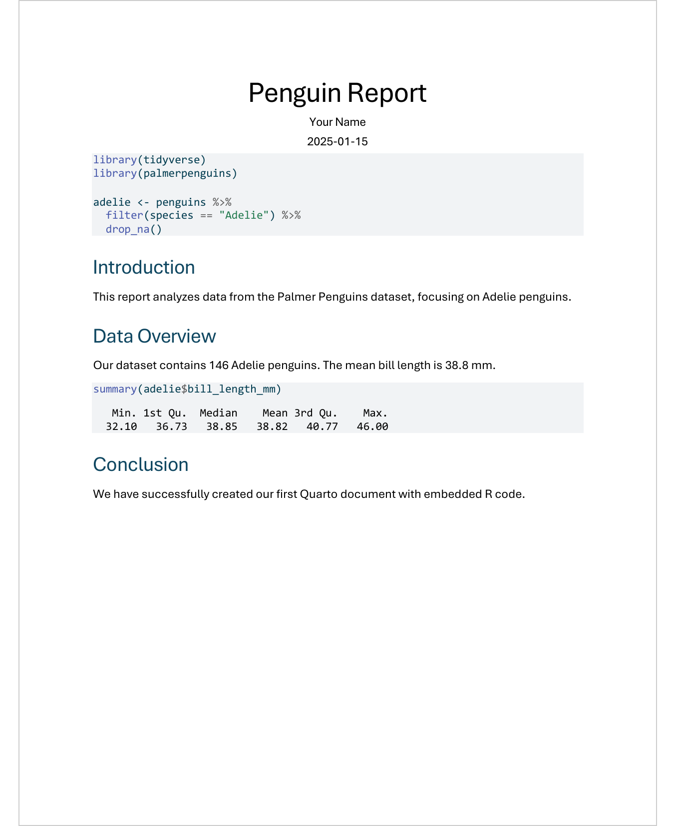
As you can see, the code, its output, and the inline values (146 penguins, 38.8 mm) all appear in the final document. It does not look very polished yet - we will fix that in the coming chapters.
- Create a new Quarto document in RStudio
- Replace the content with the example above
- Render it to Word
- Open the Word file and examine the result
- Try changing the species from “Adelie” to “Gentoo” and re-render - notice how all numbers update automatically
What is next
The rendered Word document works, but it probably does not look very polished yet. The R output appears as plain text, and the formatting is generic. In the following chapters, we will learn how to:
- Control what code and output appears in the document (Chapter 3)
- Use Word templates for professional formatting (Chapter 4)
- Create beautiful tables with flextable (Chapter 5)
- Add well-formatted plots (Chapter 6)
Citation
@online{schmidt2026,
  author = {{Dr. Paul Schmidt}},
  publisher = {BioMath GmbH},
  title = {2. {Your} {First} {Quarto} {Document}},
  date = {2026-06-08},
  url = {https://biomathcontent.netlify.app/content/quarto/02_first_document.html},
  langid = {en}
}